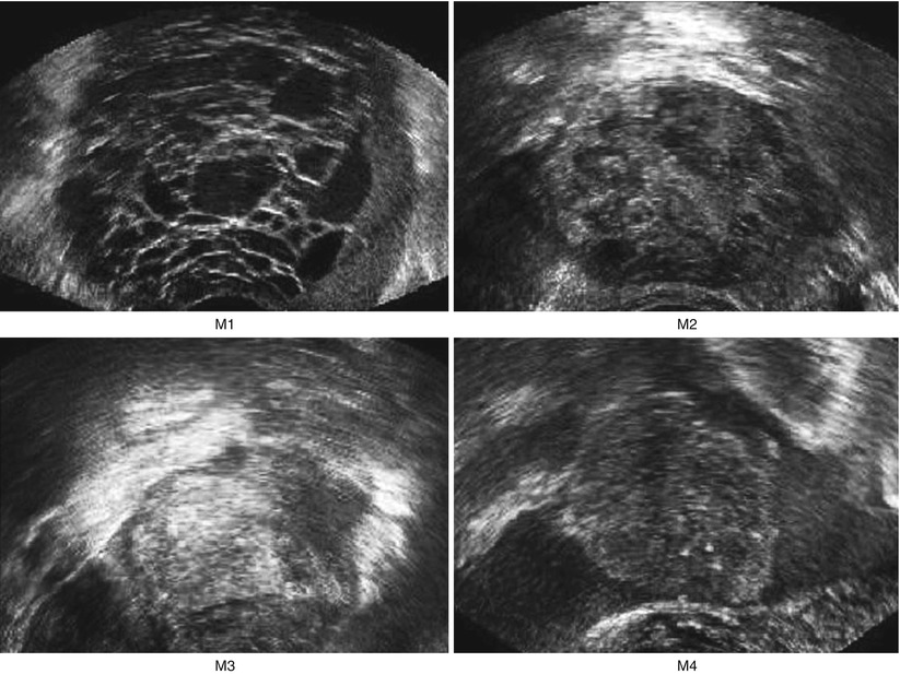
Fig. 1
Ultrasound images of the ovary: (B1–B4) benign conditions (M1–M4) malignant tumor
Methods
Figure 2 depicts the general block diagram of the proposed CAD technique for ovarian cancer detection. The dataset is split into a training set and a test set. The training set images are used to develop the classifiers. The classifiers are evaluated using the test set to simulate a real-time diagnosis scenario. In Fig. 2, steps involved in the off-line training procedure are shown in the blocks outside the shaded rectangular box, and the blocks inside the shaded box indicate the steps in the online real-time system. In the off-line training system, texture features based on Local Binary Patterns (LBP) and Laws Texture Energy (LTE) are extracted from the images in the training database. Only highly discriminative features are selected. These features and the ground truth of whether the training images are benign or malignant are used to train the support vector machine (SVM) classifier. The outputs of this off-line training system are the SVM classifier parameters that are tuned to accurately predict the class labels (benign or malignant) given the input significant features. To test this built classifier, we extract the significant features from the test set images and apply the SVM classifier parameters on them to determine the class. The classifier performance is evaluated using performance measures such as sensitivity, specificity, accuracy, and PPV.
Fig. 2
Block diagram of the proposed system for ovarian cancer detection; the blocks outside the dotted shaded rectangular box represent the flow of off-line training system, and the blocks within the dotted box represent the online real-time system
In the remainder of this section, we describe the LBP and LTE texture features, the SVM classifier, and the feature selection test (t-test) used in this work.
Feature Extraction
Local Binary Pattern (LBP): LBP [13] was initially proposed as an efficient texture operator which processes the image pixels by thresholding the 3 × 3 neighborhood and by representing the resultant label as a binary number. The histogram of these labels was used as a texture descriptor. Subsequently, the LBP operator was extended to neighborhoods of various sizes [14]. LBP has been successfully applied to a wide range of different applications from texture segmentation [15] to face recognition [16]. The LBP feature vector is determined using the following steps:
where

(a)
Consider a circular neighborhood around a pixel. P points are chosen on the circumference of the circle with radius R such that they are all equidistant from the center pixel. Let g c be the gray level intensity value of the center pixel. Let g p , p = 0, …, P−1, be the gray level intensity values of the P points. Figure 3 depicts circularly symmetric neighbor sets for different values of P and R.
Fig. 3
Circularly symmetric neighbor sets for different P and R. The center pixel denotes g c and the surrounding pixels depict g p , p = 0,…, P−1; left: P = 8, R = 1, middle: P = 16; R = 2; right: P = 24, R = 3
(b)
These P points are converted into a circular bitstream of 0’s and 1’s according to whether the intensity of the pixel is less than or greater than the intensity of the center pixel. For example, the value of the LBP code of the center pixel (x c , y c ) with intensity g c is calculated using the following equation.
(1)
In their subsequent study, in order to reduce the length of the feature vector, Ojala et al. [14] introduced the concept of uniformity. This concept is based on the fact that some binary patterns occur more commonly than others. Each pixel is classified as uniform or nonuniform and uniform pixels are used for further computation of the texture descriptor. These uniform fundamental patterns have a uniform circular structure that contains very few spatial transitions U (number of spatial bitwise 0/1 transitions). Generally, an LBP is called uniform if the binary pattern contains at most two bitwise transitions from 0 to 1 or vice versa when the bit pattern is traversed circularly. Some examples of uniform patterns are: 00000000 (0 transitions), 01110000 (2 transitions), and 11001111 (2 transitions). Thus, a rotation invariant measure called LBP P, R using the uniformity measure U ≤ 2 is calculated based on the number of transitions in the neighborhood pattern (Eq. 2).
where
(2)
Multi-scale analysis of the image using LBP is done by choosing circles with various radii around the center pixels and then constructing separate LBP image for each scale. In our work, energy and entropy of the LBP image, constructed over different scales (R = 1, 2, and 3 with the corresponding pixel count P being 8, 16, and 24, respectively, see Fig. 3), were used as feature descriptors. Thus, there were in all six LBP-based features. For example, LBP entropy obtained using R = 1 and P = 8 is denoted as LBP 18 Ent and LBP energy obtained using R = 1 and P = 8 is denoted as LBP 18 Ene.
Laws Texture Energy (LTE): Laws empirically determined that several masks of appropriate sizes were useful for discriminating between different kinds of texture [17]. The method is based on applying such masks to the image and then estimating the energy within the pass region of filters [17]. The texture energy measures are obtained by using three 1D vectors: L3, E3, and S3 that describe the following features: level, edge, and spot, respectively. L3 = [1, 2, 1], E3 = [−1, 0, 1], S3 = [−1, 2, −1]. By convolving any vertical 1D vector with a horizontal one, nine 2D masks of size 3 × 3, namely, L3L3, L3E3, L3S3, E3E3, E3L3, E3S3, S3S3, S3L3, and S3E3, are generated. For example,
(3)
All these masks, except L3L3, have zero mean. We used these eight zero-sum masks numbered 1–8. To extract texture information from an image I(i, j), the image is first convolved with each 2D mask. For example, if we used E3E3 to filter the image I(i, j), the result was a texture image TIE3E3 as shown below.
(4)
To make the resultant images contrast independent, the texture image TIL3L3 was used to normalize the contrast of all other texture images as shown in Eq. 5.
(5)
The resultant normalized TIs were passed to texture energy measurements (TEM) filters which consisted of a moving nonlinear window average of absolute values (Eq. 6).
(6)
Thus, in this feature extraction process, the image under inspection is filtered using these eight masks, and their energies are computed and used as the feature descriptors [18]. A total of eight features were extracted, one using each of the eight masks, denoted by LTE 1 Ene, etc. A more detailed analysis of applications of Laws texture can be found in the recent book by Mermehdi et al. [19].
Support Vector Machine Classifier
Support vector machine (SVM) [20–22] is a supervised learning-based classifier that uses the input features from the two classes to determine a maximum margin hyperplane that separates the two classes. The hyperplane is determined in such a way that the distance from this hyperplane to the nearest data points on each side, called the support vectors, is maximal. Consider two-class classification using a linear hyperplane of the form
where ϕ(•) denotes the feature transformation kernel, b is the bias parameter, and w is the normal to the hyperplane. The training data consists of the input feature vectors x and the corresponding classes c. c = −1 for benign class and +1 for malignant class. At the end of the training, the optimal values for the parameters w and b are determined. During the testing phase, the new feature vector is classified based on the sign of y obtained using Eq. 7. The perpendicular distance to the closest point from the training data set is the margin, and the objective of training an SVM classifier is to determine the maximum margin hyperplane and also to assign a soft penalty to the samples that are on the wrong side of the margin. The problem becomes an optimization problem where we have to minimize
where ξ i are the penalty terms for samples that are misclassified, C is the regularization parameter which controls the tradeoff between the misclassified samples and the margin. The first term in Eq. 8 is equivalent to maximizing the margin. This quadratic programming problem can be solved by introducing Lagrange multipliers a n for each of the constraints and solving the dual formulation. The Lagrangian is given by
![$$ \begin{array}{c}L\left(w,,b,,a\right)=\frac{1}{2}\parallel w\parallel {\kern0.1em }^2+C{\displaystyle \sum}_{i=1}^N{\xi}_i\\ {}-{\displaystyle \sum}_{i=1}^N{a}_i\left[{c}_iy\left({x}_i\right)-1+{\xi}_i\right]-{\displaystyle \sum}_{i=1}^N{\mu}_i{\xi}_i\end{array} $$](/wp-content/uploads/2016/09/A301939_1_En_25_Chapter_Equ9.gif)
where a i and μ i are the Lagrange multipliers. After eliminating w, b, and ξ i from the Lagrangian, we obtain the dual Lagrangian which we maximize.
(7)
(8)
(9)
(10)
The predictive model is now given by
and b is estimated as
(11)