Ultrasound Evaluation of Normal Fetal Anatomy

Outline
Superficial Anatomy of the Fetus, 161
Musculoskeletal System, 161
Cardiovascular System, 183
Gastrointestinal System, 191
Respiratory System, 197
Genitourinary System, 199
Central Nervous System, 200

Summary of Key Points

•

Continued advancement of ultrasound technology including increase in frequency and choice of focal position have improved visualization of fetal anatomy and therefore have also increased the required anatomic knowledge of these structures for those performing and interpreting fetal sonograms.
•

Superficial anatomy of the fetus can be delineated with either two-dimensional or three-dimensional sonography and can be useful in confirming normal formation of facial structures and genitalia.
•

Fetal skeletal structures are the earliest recognizable fetal features, and their sonographic evaluation is highly dependent on the position of the fetus.
•

Identification of a normal three-vessel umbilical cord and normal portal venous anatomy is useful in determining whether cardiovascular development is normal.
•

The liver is the largest gastrointestinal organ and is the largest contributor to the size of the abdominal circumference.
•

The lungs become more echogenic later in pregnancy; however, the change is not related to lung maturity.
•

Kidneys grow throughout pregnancy, with a ratio of kidney circumference to abdominal circumference of 0.27 to 0.30.
•

The calvaria can obscure the portion of the brain nearest the transducer. Bone-free windows through the fontanelles can be used to increase visualization, and when one hemisphere is not well seen, symmetry is assumed unless images prove otherwise.

Our understanding of normal fetal anatomy as seen on sonograms continues to evolve. Instrumentation has improved steadily, yielding both improved and more consistent image quality. Among the most significant advances in fetal imaging has been the ability to choose the depth of the zone of best focus of the ultrasonic beam and to select frequency without changing transducers. With these capabilities, the area of anatomy being observed can be consistently inspected with the focused portion of the beam at an optimal frequency, both highly significant advantages. Recent technologic advances allow imaging at higher frequencies than a mere decade ago.

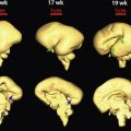
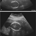
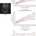
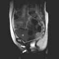
In addition to these technologic advances, sonologists have gradually improved their understanding of the anatomy portrayed on in utero sonograms. Unquestionably, clearer images have led the way to our improved understanding, but other factors have been involved; not the least of these has been the surge in ultrasonic imaging of premature neonates. These tiny neonates are the equivalent of second trimester fetuses as early, at times, as 24 weeks’ gestation. Visualization of their brains ( Fig. 8-1 ) and abdominal ( Fig. 8-2 ) anatomy in the ex utero environment, which permits the use of higher frequency transducers, a greater selection of planes of section, and comparison with other imaging modalities, has done much to improve our understanding of fetal anatomy. This information can be, to a large extent, extrapolated to younger fetuses. As well, as magnetic resonance imaging (MRI) continues to be a growth area in fetal imaging, our ability to compare sonographic anatomy of the fetus with that portrayed on MR imaging further enhances our understanding of fetal sonographic anatomy ( Fig. 8-3 ).

The ability of sonography to detect intrafetal structures is a balance between spatial resolution and contrast. This balance, however, strongly favors contrast as the more important aspect of perception. For example, a large white dot on a white wall is difficult or impossible to see because no contrast differential exists even though the eye can spatially resolve easily a tiny black dot (high contrast) on the same wall. Structures possessing high levels of subject contrast can be consistently detected at a smaller size (often equating to an earlier age) than those displaying poor contrast. Although sonographic contrast agents are available for imaging in adults and children, current agents do not cross the placenta in sufficient concentration to affect fetal organs. Therefore, sonologists possess no agents to alter contrast of fetal organs and thus are totally dependent on subject contrast (inherent contrast) for visualization of internal fetal morphologic details. Clearly, spatial resolution is also a critical feature in defining morphologic structure but has not been the limiting factor in demonstrating fetal anatomy. Fortunately, sophisticated modern sonographic imaging systems have the ability to choose varying contrast settings, which enhance inherent tissue differences. An important aspect of the technical advancements allowing ever higher frequency imaging is that at higher frequencies, contrast differences between organs change, which can have diagnostic impact.

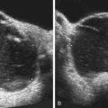
Another technology that has improved fetal imaging, particularly for earlier gestations, is the intracavitary (transvaginal) transducer. Certain aspects of fetal and even embryonic, anatomy can be seen with amazing detail ( Fig. 8-4 ). Although this methodology is crucial to modern imaging, we intend to concentrate our discussion on anatomy visualized by transabdominal transducers in fetuses beyond the 14th week. When examining later pregnancies, in the context of fetal anatomic imaging, we use transvaginal transducers predominantly to visualize the presenting part when transabdominal transducers fail to adequately image this region of the fetal anatomy (e.g., distal sacrum in a breech fetus).

Other parameters, important in fetal imaging, also cannot be controlled. Sonography is a tomographic technique. Appropriate positioning for obtaining the best tomographic plane is always desirable. However, we are unable to control fetal position to attain this end. We also cannot control maternal body habitus or the amount of amniotic fluid, both of which may dramatically alter our ability to discern fetal anatomy. Despite these problems, a large number of fetal structures are consistently visible sonographically.

High-resolution, real-time scanners with their flexible approach to imaging are mandatory for modern fetal sonography. In the following sections, various aspects of fetal anatomy are detailed as seen on such instrumentation. An estimate is made of the ability of ultrasound instrumentation to consistently demonstrate the anatomic part under consideration as well as an attempt to estimate when the fetus has attained sufficient size such that the anatomic structure is large enough to be detected. It is important to recall that size and visualization may be relative at any given stage of development. For example, in a small fetus with a well-distended urinary bladder, identification of the bladder is relatively easy. Alternatively, identification of the bladder will be difficult in a term fetus that has recently voided. The urine, in this instance, provides the “contrast” that ordinarily makes the urinary bladder an easy structure to perceive. If this contrast agent drains away, the size of the fetus (and thus its bladder) will not rescue one from the loss of contrast. Also important is the concept that the human eye sees best in the “relative” rather than the “absolute” sense of size. Thus, in a young fetus, the cerebral ventricle is much more readily seen than in an older fetus because the relative size of the ventricle compared with overall brain size is larger early (even though the absolute size is larger later).

If the sonographer begins with a specific intent to image a particular fetal part, it is frequently possible to succeed. To accomplish this end, the sonographer must (1) assess the precise fetal position; (2) consider whether the anatomic part of interest is best visualized in planes perpendicular to the fetal long axis or parallel to the fetal long axis; and (3) adjust acoustic imaging parameters, particularly time-gain compensation, and transducer angulation to visualize the area to best advantage. Obviously, such rules are the same throughout all of sonography. The challenge of imaging intrafetal structures is to apply these rules when fetal position is changing such that the current scanning plane is no longer applicable for the part one wishes to visualize.

The flexibility offered by real-time sonographic systems enables one to survey the fetus quickly to determine precise position. Second, the sonographic tomograms, which are rapidly generated (virtually “real-time” imaging), enable one to view a large volume of the fetus with closely spaced sections. Such a rapid look at many contiguous tomograms eliminates one of the basic flaws of tomographic imaging of a moving target. Finally, fetal movements are viewed directly, which enables one to quickly reorient the transducer to the optimal plane of section to image the structure of interest. As digital image storage and viewing continues to expand, cine clip technology has greatly improved the capture and viewing of many fetal parts, especially those that are in motion, like the heart. Surprisingly, many imaging groups fail to take advantage of cine technology when recording fetal examinations. This immensely powerful technology should not be left on the sidelines by imaging specialists.

Currently, three-dimensional imaging systems have reached a clinically relevant stage of development. These instruments depend on volume imaging . That is, a volume of tissue within the fetus is insonated and the data are gathered in the processing computer. From this volume, three-dimensional images are generated. Of perhaps greater importance in the future, individual planes of section in virtually any orientation can be computed. When and if it becomes possible to generate equivalent planar images to those obtained with a hand-held transducer, the current method of “fluoroscopic” sonography, the entire nature of sonography will change. The technical challenges of sonography will be greatly reduced ( Fig. 8-5 ).

Fetal parts of interest to the sonologist fall into three major categories of subject contrast that subsequently determine the relative ease with which the structure is sonographically visible: (1) structures that generate high-amplitude reflections (e.g., ossified bones, submucosa of fetal bowel, leptomeninges); (2) structures that generate no internal echoes (e.g., fluid-containing viscera); and (3) structures that generate midrange gray echoes (e.g., the parenchymal organs such as the lungs, brain, spleen, liver, kidneys, and muscles). The categories are listed from most visible to least visible. Within the last category, one may anticipate seeing a spectrum of gray shades that will enable distinction between parenchymal organs and intraorgan components. For example, the medullary portions of the fetal renal parenchyma generate lower amplitude internal echoes than do the surrounding cortical tissues and Bertin septa, thus enabling recognition of this separate component of renal tissue ( Fig. 8-6 ). Modern imaging systems enable distinctions previously not possible. An example from a relatively common pathologic circumstance is the apposition of the herniated spleen against the lung in left congenital diaphragmatic hernia. Previously these organs “blended” together, but currently they are readily discriminated, resulting in better estimations of residual lung volume in affected fetuses ( Fig. 8-7 ).

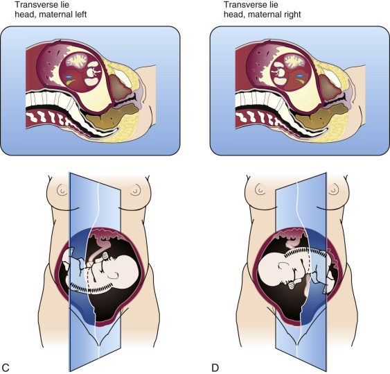
A feature of critical importance for organ imaging is the fetal position. A prone fetus is in an optimal position for imaging the kidneys, ordinarily difficult to perceive, but in a poor position to demonstrate the urinary bladder, which is usually easy to image. Determination of fetal position should be accomplished in all obstetric sonographic examinations from the second trimester onward. The fetal position should be determined as precisely as possible before an interpretation of fetal anatomy is begun, because the position of a structure will often influence our interpretation. The general fetal orientation is first assessed (e.g., cephalic, breech, oblique, or transverse). Once this is determined, the location of the fetal spine is noted. If, for example, the fetal spine is on the maternal left side and the fetus is in a cephalic presentation, one can judge that the fetus is lying on its left side ( Fig. 8-8 ). Conversely, if the fetus is breech, then it must be lying on its right side. The reverse is the case for breech and cephalic fetuses when the fetal spine lies on the maternal right side. In the transverse or oblique fetal positions the same rules apply but with a different orientation.

Such an analysis of fetal position is vital for proper interpretation of abdominal and thoracic situs (now a requirement of the AIUM/ACR/ACOG [American Institute of Ultrasound in Medicine/American College of Radiology / American College of Obstetricians and Gynecologists] practice guidelines for second and third trimester obstetric sonograms) and for identification of abnormal fetal structures. For instance, a rounded, fluid-filled structure in the left posterior portion of the upper fetal abdomen may be assumed to represent the fundus of the fetal stomach. However, a structure of identical appearance but located on the right side of the upper fetal abdomen must be interpreted as a pathologic lesion or an abnormality of situs.

It is important to recall that pathologic structures are frequently more visible than their normal counterparts (e.g., dilated small bowel loops are easier to detect than normal small bowel loops). However, it is even more important to keep in mind that the most difficult pathologic observation is to recognize the absence of a structure that ordinarily could be visualized (i.e., a missing portion of an extremity or the inability to see the stomach when esophageal atresia without tracheoesophageal fistula is present).

Superficial Anatomy of the Fetus

Routine sonography for obstetric indications in many cases does not require a survey of superficial fetal structures. However, when an anomaly is suspected, a careful look at superficial features of the fetus becomes important or even mandatory. Superficial anatomy considered in this section includes the face, ears, hair, and external genitalia. Importantly, technologic advancements in three-dimensional renderings of fetal sonograms have had a dramatic impact on visualization of superficial fetal anatomy.

The fetal face can be viewed with considerable clarity with two-dimensional sonography. Expectant mothers are often surprised to see their fetus so clearly ( Figs. 8-9 to 8-11 ). The brow, cheeks, eyelids (and occasionally even eyelashes), nose, lips, and chin can be seen with consistency. The nose and lips are the more important to image in detail (to exclude clefting). The alae, column, and nares can be clearly depicted ( Figs. 8-12 and 8-13 ). The upper lip is more important diagnostically than the lower lip and fortunately easier to see. Visualization is usually good enough to identify the philtrum. The cheeks are prominent, as expected, and the subcutaneous tissues of the cheek, because of the presence of a large fat pad, are brightly echogenic ( Fig. 8-14 ). The profile is also readily demonstrated (see Fig. 8-11 ) and provides useful information about the brow (e.g., frontal bossing), chin (e.g., hypognathia), and nose (e.g., midface hypoplasia and Down syndrome).

The ears can be visualized quite well and their progressive maturation noted. The external auditory canal, helix (and antihelix in older fetuses), lobule, and tragus can be depicted ( Fig. 8-15 ), but the relative position of the ear (e.g., as in low-set ears) is difficult to judge—a task more readily accomplished with three-dimensional imaging. The ear may be protuberant and can be mistaken for an abnormality, especially an encephalocele.

When present, scalp hair is readily perceived in late fetuses. The bright linear echoes protruding from or paralleling the scalp and neck are quite conspicuous. The only benefit of recognizing hair is not to be misled into mistaking long hair for a pathologic process—namely, an encephalocele or cystic hygroma—because longer hair, wet and matted by the amniotic fluid, may trap some of the fluid between it and the skin of the occiput or neck, creating the false impression of a cystic mass in this location ( Fig. 8-16 ).

The external genitalia can be appreciated from early second trimester onward. Fetal sex can be quite accurately assigned. Ordinarily, this is not of clinical consequence. However, in certain circumstances, fetal sex should always be determined. These situations include all living twins in which a single placental site is seen or when monozygotic twinning, other than for reasons of placentation, would be considered detrimental to pregnancy outcome. All fetuses with suspected lower urinary tract obstruction should have fetal sex determined because the differential diagnosis is different in males and females. Certain other circumstances would require determination of sex if karyotyping were refused or impractical to perform and cell-free DNA screening were not possible or inconclusive. These indications include, but are not limited to, risk for X-linked disorders or when Turner syndrome is suspected because of a dysmorphic feature (e.g., cystic hygroma).

Female sex should be assigned only by identification of the major and minor labia ( Fig. 8-17 ). Assigning female sex based solely on an inability to see a penis will result in many diagnostic errors. Male genitalia are readily seen ( Fig. 8-18 ). The penis and scrotum are most obvious. Testes may be seen in the scrotal sac, sometimes as early as the beginning of the third trimester (the testes are intra-abdominal during most of gestation but are only visualized in the presence of ascites). Care should be taken to image the entirety of the phallus to avoid false foreshortening. Details of the penis, including the glans, urethra, and corpora cavernosa, may be appreciated ( Fig. 8-19 ). Even the foreskin is visible in some cases.

Musculoskeletal System

Real-time ultrasonography provides the most appropriate format for imaging fetal bones. The resolution and flexibility offered by such systems enable one to survey the fetal skeleton rapidly. Of all structures within the fetus, the ossified portions of the skeleton possess the highest level of subject contrast and thus are seen earlier and more consistently than any other organ system. Sonography surpasses all other imaging modalities in fetal skeletal imaging. Although radiographs of abortuses demonstrate bony morphologic appearance more advantageously than would a sonogram, the reverse is true of fetuses in the womb, where overlying maternal soft tissues and bones, fetal movement, and inappropriate fetal position degrade radiographic images of the early fetal skeleton. With volumetric imaging (three-dimensional sonography), special processing can give a more global view of fetal skeletal structures than can be achieved with two-dimensional sonography. This enhances the image and diagnostic process for assessment of both normal and pathologic findings ( Fig. 8-20 ).

Fetal position dramatically affects visualization of the bony structures. The posterior elements of the fetal spine may be clearly imaged with the fetus in a prone or decubitus position but are difficult to image when the fetus is supine. Similarly, the extremities are imaged to excellent advantage when floating freely in the amniotic fluid, yet when tucked under the fetus an extremity will be quite difficult to adequately assess.

Despite these potential problems, fetal skeletal structures remain the earliest and most readily recognized fetal anatomic structures. The earliest structures seen with consistency are the ossification centers of the maxilla, mandible, and clavicle, the first bones of the human body to ossify. The calvaria can be imaged from the late first trimester onward. The same is true of the long bones of the upper and lower extremities ( Fig. 8-21 ). Visibility of bony detail rapidly increases, and by 15 to 16 menstrual weeks (sometimes earlier) even phalanges can be visualized. Bones as small as 2 to 3 mm can be consistently imaged by sonography, provided that no unusual impediments to the scanning procedure exist ( Fig. 8-22 ). Many specific bony structures can be depicted. Bones in both the appendicular and axial skeleton are well imaged.

Sonography has the capacity to visualize not only the ossified portions of the fetal skeleton but also the cartilaginous portions. Bones entirely in cartilage can be seen sonographically ( Fig. 8-23 ). Cartilaginous ends of the long bones may be seen by the early second trimester. It is also important to recognize that the full thickness of the ossified diaphysis of long bones is not seen sonographically. This is due to acoustic shadowing. The cartilaginous ends of long bones help us to recognize this aberration. By matching up the width of the epiphysis, the full thickness of which can be seen, with the apparent width of the bony diaphysis, it is clear that they are unequal ( Figs. 8-24 and 8-25 ). This observation helps to eliminate perceptual errors that can lead to erroneous diagnoses. For example, the inability to see the full thickness of the femoral diaphysis creates the impression that the fetal femur farther from the transducer is bowed ( Fig. 8-26 ). This error is caused by visualization of only the medial cortex of the femoral diaphysis (which is normally curved) ( Fig. 8-27 ). However, the inability to visually correct this normal curvature by simultaneous observation of the straight lateral cortex may cause a perceptual error.

The majority of the bones of the appendicular skeleton can be seen in the early to mid–second trimester, although phalanges may be difficult to perceive in some instances. It is a general rule of appendicular skeletal imaging that the more proximal a bone, the more readily it is identified. This rule in one sense is untrue of the hands and feet, where the metacarpals and metatarsals are seen more readily and earlier than either the carpal or tarsal bones ( Figs. 8-22 and 8-28 ). This is because the metacarpals and metatarsals are well ossified at 4 months, whereas the carpals and tarsals (except for the tarsal calcaneus and talus) remain cartilaginous throughout pregnancy. The tarsal calcaneus and talus ossify between the 5th and 6th months, whereas the remaining tarsals and carpals do not ossify until after birth ( Figs. 8-29 and 8-30 ).

The scapula ( Figs. 8-31 and 8-32 ), clavicle ( Fig. 8-33 ), humerus ( Figs. 8-31 and 8-34 ), radius ( Fig. 8-35 ), ulna (see Figs. 8-34 and 8-35 ), metacarpals (see Figs. 8-22 and 8-35 ), and phalanges ( Fig. 8-36 ) can be imaged in most cases. Interestingly, the clavicle may be difficult to see, presumably because of the flexed position of the fetal neck, which draws the calvaria into an obscuring position. Nonetheless, if one desires to see the clavicle, this can nearly always be accomplished. Measurements exist for normal clavicular length at various gestational ages. Similarly, the femur ( Figs. 8-37 to 8-40 ), tibia ( Figs. 8-41 and 8-42 ), fibula (see Fig. 8-41 ), metatarsals (see Figs. 8-28 and 8-29 ), and phalanges (see Fig. 8-28 ) of the lower extremity can be appreciated well sonographically. The figures demonstrating the hip joint, femur, and knee (see Figs. 8-37 to 8-41 ) demonstrate the remarkably detailed anatomy that can be achieved with high-resolution sonography.

The simplest way to identify the types of long bones of the extremity viewed on the sonogram is to obtain planes of section that traverse the short axis of the limb. Sonograms obtained in such a plane through the forearm and lower leg will demonstrate two bones. In the lower leg, the more lateral bone is the fibula, and the medial bone is the tibia (see Fig. 8-41 ). This method works as well in the forearm but is less precise because pronation may cause the radius and ulna to “cross.” In the normal fetus, the tibia and fibula and radius and ulna end at the same level distally (see Fig. 8-35 ). Proximally, the ulna is longer than the radius (see Fig. 8-34 ) and the tibia is longer than the fibula. This allows both ready differentiation of the tibia and fibula in the lower extremity and of the radius from the ulna in the upper extremity. Knowledge that both paired long bones of the upper and lower extremity end at the same level distally is important in assessing possible limb reduction abnormalities.

The hand can be assessed more critically than the foot. With patience one can usually discern all four fingers and the thumb. The hand is frequently clenched in a fist-like fashion, which can complicate the counting of fingers. However, even under this circumstance, one can frequently make the necessary observations. The toes, although smaller than the fingers, can be seen relatively well with modern equipment (see Figs. 8-28 and 8-30 ). If difficulty arises, it is usually the functionally less important fourth and fifth toes that are not seen.

It is possible in the late third trimester fetus to identify the distal femoral ( Figs. 8-25 and 8-43 ) and proximal tibial (see Fig. 8-43 ) epiphyseal ossification centers. Ossification of these epiphyses, as seen on radiographs, is known to be an indicator of fetal maturity. Identification of the epiphyseal ossification centers about the knee provides a different type of parameter that sonologists can use in the assessment of gestational age in the third trimester of pregnancy. In general, visualization of a distal femoral epiphyseal ossification center indicates a gestational age of at least 33 weeks ( Figs. 8-44 to 8-46 ). Similarly, the same data suggest that demonstration of the proximal tibial epiphysis indicates a gestational age of at least 35 weeks. These ossification centers appear earlier, on average, in female fetuses (see Fig. 8-45 ). The size of the distal femoral ossification center correlates with late gestational age (see Fig. 8-46 ). The proximal humeral epiphyseal ossification center is usually the last of the secondary ossification centers to ossify and generally can be seen at a gestational age of 38 weeks or later.

As stated earlier, many bones of the fetal appendicular skeleton are entirely cartilaginous. Some of these still can be imaged sonographically. For example, the patella, which does not begin to ossify until after birth, can be seen rather commonly (see Figs. 8-23 and 8-25 ). All of the carpal and most of the tarsal bones are entirely cartilaginous (see Figs. 8-22, 8-28, 8-29, and 8-35 ). The carpal bones cannot be seen discretely. Rather, they are perceived as a conglomerate hypoechoic band spanning the gap from the distal radius and ulna to the proximal metacarpal ossification centers (see Fig. 8-35 ). This gap includes the cartilaginous epiphyses of the long bones as well. Conversely, some of the tarsal bones can be discretely identified from time to time (see Figs. 8-28 and 8-29 ). These include, most notably, the early calcaneus and talus (before 24 weeks) and the tarsal navicular and cuboid throughout gestation.

Visualization of the cartilaginous ends of the long bones assists in their measurement in two ways. The measurement of fetal long bones is confined to the ossified portion. A potential error is to foreshorten the bone by failing to obtain the plane of section through the true long axis of the bone. To avoid underestimating length, this shortcoming is often compensated for by assuming the “longest” measurement obtained in several attempts to be the most accurate, an assumption that can lead to serious overestimates, as is discussed shortly. However, if both cartilaginous ends of the desired bone to be measured are seen, this guarantees that the plane of section has passed through the longest axis of the bone ( Fig. 8-47 ). The only remaining task to minimize error is to accurately position measurement cursors at the ends of the bone.

Another common misconception in measurement of the femur is that no other tissue in proximity to the bony termination will yield an echo of equal brightness to the bone. Thus, one should always place measurement cursors from the edge of the distal brightest reflection to the edge of the proximal brightest reflection. This longstanding belief is unfortunately untrue, especially in older fetuses, although younger fetuses are not exempt from this potentially significant error in femur length estimation. Figure 8-48 demonstrates that a nonosseous, but nonetheless equally bright, reflection is returned from tissues distal to the epiphyseal plate but in immediate contiguity with the distal femoral metaphysis. This is called the distal femoral point for lack of a more precise anatomic term. That this “point” is not part of the ossified femur can be determined by noting its relationship to the cartilaginous lateral condyle. The femoral metaphysis ends at the beginning of the distal femoral epiphysis and does not overlap the edge of the epiphysis. Compare the radiograph of the fetal femur in Figure 8-27 with the sonogram of the fetal femur in Figure 8-48 . No such ossified femoral point exists.

Sonography, from time to time, demonstrates rather extraordinarily detailed anatomy of the musculoskeletal system of the extremities such as indivudal tendons and ligaments. At present, no known diagnostic usefulness for this information has been established, nor is it possible to demonstrate such structures with the consistency necessary to use their visualization in diagnostic pursuits. However, several of these remarkable features are demonstrated in Figures 8-49 to 8-51 .

Many bones or components of bones of the axial skeleton are also routinely visualized. In the skull region, one can perceive a number of bones individually or as a conglomerate. The greater wings of the sphenoid and petrous ridge are easily identified and define the anterior, middle, and posterior cranial fossae ( Fig. 8-52 ). Both orbits can be visualized without difficulty unless the more anteriorly positioned orbit severely shadows the more posteriorly positioned orbit ( Fig. 8-53 ). Standards have been established for fetal interorbital distances to evaluate hypotelorism and hypertelorism. In older fetuses, surprising detail of the intraorbital contents can be appreciated, including the wall of the globe, lens, retrobulbar fat, optic nerve, and rectus muscles ( Fig. 8-54 ). Portions of the maxilla and nearly the entire mandible can be identified, as can the bony nasal ridge (see Fig. 8-53 ). Similarly, the frontal, parietal, and squama of the temporal and occipital bones, the bones making up the calvaria, can be seen clearly. The cartilaginous zones of articulation of these bones, the coronal, sagittal, and lambdoid sutures, are commonly visible ( Fig. 8-55 ). The fontanelles may be seen as well ( Fig. 8-56 ). These anatomic features are particularly well seen in three-dimensional reconstructions of the calvaria, as demonstrated in Chapter 11 . Sutures and fontanelles function as windows for brain imaging ( Fig. 8-57 ). Although many individuals who perform sonography do not realize that they are employing sutures and fontanelles to image the fetal brain, they visually ascertain that, as they move the transducer, “fuzzy” brain images suddenly become clearer. The reason, of course, is that as they move the transducer the beam inevitably passes through a suture or fontanelle, enabling even the unsophisticated imager to take advantage of these gaps between the calvarial plates.

The ribs, spine, and pelvis are easily imaged and serve as excellent anatomic landmarks. In the pelvis, the iliac ossification centers are easily observed from the early second trimester onward (ossified at 2.5 to 3 fetal months). Ischial ossification (see Fig. 8-37 ) is present at 4 months, whereas pubic ossification is not present until 6 months.

The spine is an extremely important structure in fetal diagnosis. With the advent of maternal serum α-fetoprotein screening, as well as the concurrent development of sophisticated high-resolution ultrasound imaging technology, the potential exists to diagnose nearly all lesions of spina bifida before the 20th week of pregnancy. These changes in obstetric care mandate that the morphologic appearance of the fetal spine be well understood by sonologists. The sequence of development of ossification centers in the fetal vertebral column has been extensively studied in the past with radiologic and histologic methods. Each vertebra usually has three primary ossification centers, one for the body (centrum) and one on each side of the posterior neural arch. The centra are ossified first in the lower thoracic and upper lumbar regions followed by progressive ossification in both the cephalic and caudal directions. By contrast, and in general, the ossification centers for the posterior neural arch appear in a more standard cephalocaudal direction. The posterior neural arch first begins to ossify (sonographically recognizable high-amplitude reflections) at the base of the transverse process ( Fig. 8-58 ). Ossification proceeds from this center to progressively include the laminae and pedicles. The progression of ossification of the laminae is more important for the diagnosis of neural tube defects because spina bifida is the most consistently demonstrable dysmorphic lesion in open spinal defects. This abnormality is recognized sonographically by an abnormal outward flaring of the posterior neural arch ossification centers.

Varying degrees of maturation of spinal ossification are present at differing levels of the spine when we are most frequently called on to assess normality of the fetal spine. Although there are some exceptions as noted previously, ossification in the neural arch first appears at the base of the transverse process. Early posterior neural arch ossification then progresses anteriorly into the pedicles, also contributing a portion of the vertebral body, and posteriorly into the laminae. Additionally, craniocaudal extension into the articular processes and lateral extension into the transverse processes occur. Because the critical observation in the diagnosis of open spinal neural tube defects is the demonstration of spina bifida (seen as an outward flaring of the posterior arch ossification centers), the ideal situation to confirm normality is to observe the antithesis of this pathologic state (i.e., inward angulation of the laminae). This is readily acheived when visible ossification is present in the normal laminae ( Fig. 8-59 ). Unfortunately, there is insufficient ossification of the laminae to perceive inward angulation of the posterior neural arch ossification centers in the lower spine to confirm normality of the fetal spine during the crucial stage of gestation when this sonographic diagnosis must be made (18 to 22 menstrual weeks) (see Fig. 8-58 ). This is particularly important when considering the most common location of such lesions (i.e., lumbar and sacral regions). Easily identifiable ossification of the laminae is visible in the cervical region in all fetuses by 18 to 19 menstrual weeks, whereas thoracic ossification of the laminae is only partially visible during 18 to 19 menstrual weeks. There is no ossification of the laminae in the lumbar or sacral regions of fetuses examined before 19 menstrual weeks (see Fig. 8-58 ). The thoracic vertebrae consistently demonstrate partial ossification of the laminae in the range of 20 to 22 weeks; the lumbar region does not demonstrate a similar degree of ossification until 22 to 24 weeks ( Fig. 8-60 ). The sacral spine reveals no evidence of ossification in the laminae before 22 weeks. Only after 25 weeks is there consistently recognizable ossification of the arch in the sacral region ( Fig. 8-61 ). Fetal position (either prone or decubitus) does not appear to affect appreciably the ability to discern the degree of neural arch ossification, although the prone position usually results in the clearest images ( Fig. 8-62 ). If the fetus is supine, a critical examination of the posterior neural arch cannot be accomplished ( Fig. 8-63 ).