Segmentation of Pelvic Structures from CT Scans for Planning in Prostate Cancer Radiotherapy

Fig. 1

Workflow for traditional prostate cancer image-guided radiation therapy. The prescribed radiation dose for EBRT is generally delivered over several weeks in small daily amounts (fractions)

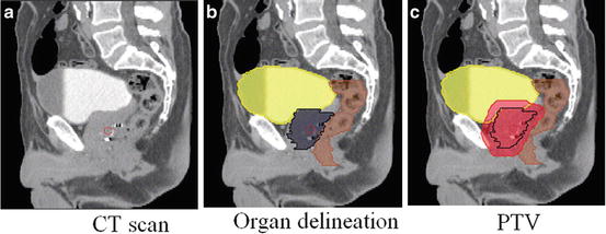
Fig. 2

Sagittal views of a male pelvis showing the original CT scan (a) with overlaid delineations of the bladder, rectum and prostate (b) and with the planning target volume (PTV) (c) defining the area which will receive the prescribed radiation dose

The next step is the use of computer planning tools to determine the directions, strengths, and shapes of the treatment beams which will be used to deliver a prescribed dose to the defined target while minimizing the dose to the normal tissues, according to a certain number of recommendations (e.g., [9]). Thus, a treatment plan consists of dose distribution information over a 3D matrix of points overlaid onto the individual’s anatomy. Dose volume histograms (DVHs) summarize the information contained in the 3D dose distribution and may serve as tools for quantitative evaluation of treatment plans. The International Commission on Radiation Units and Measurements (ICRU) 50 and 62 reports define and describe several target and critical structure volumes that aid in the treatment planning process and that provide a basis for comparison of treatment outcomes. For example, to comply with ICRU recommendations for prostate, 95 % of the PTV is irradiated with at least 95 % of the prescribed dose. For the rectal wall the maximal dose should be less or equal than 76 Gy and the irradiated volume at 72 Gy must be less than 25 %. Finally, during the dose delivery step, which may last several weeks, the patient is carefully positioned at the accelerator and the treatment is performed according to the planning. A frequent method to align the patient for treatment is to use small implanted fiducial markers in the prostate. These are visible under X-ray imaging and show precise prostate position within the body. Image guidance may also be used to align the treatment target each day for the entire course (Fig. 3).

Fig. 3

Typical intensity modulated radiation therapy (IMRT) plan (axial, coronal, and sagittal views) showing iso-dose curves and the (PTV), obtained after organ delineations

One of the main challenges in prostate radiotherapy is to control the tumor, by accurately targeting the prostate, while sparing neighboring organs at risk (OAR) (bladder and rectum). Several strategies have been developed in order to improve local control, particularly by increasing the radiation dose with highly conformal techniques demonstrating a strong dose-effect relationship [10]. The precision of treatment delivery is steadily improving due to the combination of intensity modulated RT (IMRT) and image-guided RT (IGRT) and intraprostatic fiducial markers. New delivery systems are also populating clinical centers (ARC-Therapy, cyberknife). Hence, the possibilities for achieving better control by increasing the dose are within reach. However, dose escalation is limited by rectal and urinary toxicity [11, 12]. Toxicity events (incontinence, rectal bleeding, stool lose) are frequent with standard prescribed doses (70–80 Gy) and may even significantly increase for higher doses [13]. Thus, accurate delineation of both prostate and OARs (i.e., bladder, rectum) from planning images are crucial to exploit the new capabilities of the delivery systems [14]. Identifying the boundaries of pelvic structures are of major importance not only at the planning step, but also in other radiotherapy stages such as patient setup correction, accumulating dose computation when IGRT is used [15, 16], or for toxicity population studies [17] (Fig. 4).

Fig. 4

Axial view of manual segmentation of bladder, prostate, and rectum overlaid on CT scan

Nowadays, the organ contouring tasks are mainly carried out manually by medical experts. However, the CT offers poor soft tissue contrast and therefore segmenting pelvic organs is highly time-consuming (between 20 and 40 min to delineate each). Manual contouring requires training and is prone to errors, especially in the apical and basis regions [18, 19]. These uncertainties lead to large intra- and inter-observer variation [20] and may impact treatment planning and dosimetry [19, 21]. Previous studies, for instance, have reported a prostate delineation variance of 20:60 % [20]. For the rectum and bladder this difference may be as high as 2.5 to 3 % [19]. Although improved organ contrast may be obtained with Magnetic Resonance Images (MRI), and several studies are in progress to introduce MRI in the radiotherapy planning [22, 23], CT scans are still required to perform this task since dose computation relies on electron density.

Therefore, there is a strong case for more reliable semi- or fully automatic CT segmentation techniques. When dealing with automatic segmentation methods for prostate cancer treatment, there are several difficulties which may arise. Firstly, there is a poor contrast between prostate, bladder, and rectum and, secondly, there may exist a high variability in the amount of bladder and rectum filling. These challenges restrict the use of classical intensity-based segmentation methods. In addition the high intra- and interindividual variability may cause model-based methods to fail [24] (Fig. 5).

Fig. 5

Two examples of pelvic structures in CT (sagittal views). The poor contrast between structures hampers organ segmentation

Atlas-based approaches are common methods for organ segmentation, not only for obtaining a final contour, but also to provide initial organ positions for further segmentation algorithms. In atlas-based methods a precomputed segmentation or prior information in a template space is propagated towards the image to be segmented via spatial normalization (registration). These methods have been largely used in brain MRI [25, 26], head and neck CT Scans [27–29], cardiac aortic CT [30], pulmonary lobes from CT [31], and prostate MR [32, 33]. In the atlas-based methods image registration is a key element, as label propagation relies on the registration of one or more templates to a target image.

In this chapter a brief overview of image registration and atlas methods will be provided. Atlas-based methods which can perform the segmentation of the individuals’ pelvic structures, prostate, and OAR from CT scans will be discussed and evaluated against clinical datasets.

Image Registration

Introduction

Atlas-based segmentation is heavily dependent on the quality of image registration. Medical image registration involves determining the spatial transform which maps points from a moving image to homologous points on an object in a fixed image. The general idea of the registration may be summarized as in Fig. 6.

Fig. 6

Computerized registration framework

The basic input data to the registration process are two images: one is defined as the fixed image F(X) and the other as the moving image M(X). The output of the registration is a spatial transformation T allowing the warping or the alignment of the moving image, on the fixed image, according to a similarity metric.

As depicted in Fig. 6, there are four main components involved in image registration: a similarity measure between two images; the transformation model used to map points between images; a method to find the optimal transform parameters; and finally an interpolator to calculate moving image intensities at non-grid positions [20].

In this sense, registration may be seen as an optimization problem

${\widehat{T}}_{\varTheta }= \arg \underset{T_{\varTheta }}{ \min }C\left({T}_{\varTheta };F(x),M(x)\right)$

(1)

aimed at estimating the spatial mapping that better align the moving image with the fixed image according to a cost function:

$C=s\left(F(x),T\left(M(x)\right)\right)$

(2)

where s(F(x), T(M(x)) is the similarity which provides a measure of how well the fixed image is matched by the transformed moving image. This measure forms the quantitative criterion to be optimized over the search space defined by the parameters of the transform. The similarity may lie on control points, features, anatomical structures, intensities, etc. Here, we restricted the study to the intensity similarity metrics.

Transform

The transform component T(X) represents the spatial mapping of points from the fixed image space to points in the moving image space. The transformation model can either apply to the entire volume (global) or to each voxel (local).

The two global methods are: rigid registration which allows only rotations and translations; and affine registration which extends rigid registration with the addition of skew and scaling parameters.

Deformable (also known as nonrigid or nonlinear) registration affects individual voxels within the volume. This enables the matching of soft tissues which may deform between scans (e.g., a patient’s bladder on two CBCT volumes) or when performing interindividual mapping. Typically a regularization constraint is also implemented to constrain the allowable solution space. Deformable methods can be complex and difficult to validate [34]. Common deformable transforms include BSpline free form deformation (FFD) [35], thin plate splines [36], and optical flow-inspired approaches (Demons algorithm) [37]. The output from deformable registration is generally a volume (the deformation field) which contains displacement vectors for each voxel as illustrated in Fig. 7.

Fig. 7

Example of a nonlinear transformation (b) obtained when registering the moving image (a) into the space of the fixed image (c)

Image Similarity Metrics

When the similarity between two images is based on intensity levels, several metrics can be considered [38]. These can be computed via their voxel-wise differences, for example, with the sum of squared differences (SSD), or via the cross-correlation (CC) or the mutual information (MI). These metrics are computed over the whole image as follows:

$\mathrm{SSD}=\frac{1}{n}\sqrt{{\displaystyle \sum_i{\left(F\left({x}_i\right)-T\left(M\left({x}_i\right)\right)\right)}^2}}$

(3)

where F(x _i) is the fixed image and T(M(x _i)) represents the transformed moving image. The CC as

$\mathrm{CC}=\frac{{\displaystyle \sum_i\left(F\left({x}_i\right)-\overline{F}(x)\left)\right(T\left(M\left({x}_i\right)\right)-T\left(\overline{M}(x)\right)\right)}}{\sqrt{{\displaystyle \sum_i{\left(F\left({x}_i\right)-\overline{F}(x)\right)}^2}}\sqrt{{\displaystyle \sum_i{\left(T\left(M\left({x}_i\right)\right)-T\left(\overline{M}(x)\right)\right)}^2}}}$

(4)

and the MI, computed as

$\mathrm{MI}\left(F,M\right)=H(F)+H(M)-H\left(F,M\right)$

(5)

where H(x) is the individual entropy of an image x, given by

$H(F)=-{\displaystyle \sum_ip}(i) \log p(i)$

(6)

and

$H\left(F,M\right)=-{\displaystyle \sum_{i,j}p}\left(i,j\right) \log p\left(i,j\right)$

(7)

is the joint entropy and p the joint probability. The idea behind the term−H(F, M) is that maximizing MI is related to minimizing joint entropy. A more robust version of the MI is the normalized mutual information (NMI) proposed by Studholme et al. [39] and computed as

$\mathrm{NMI}\left(F,M\right)=\frac{H(F)+H(M)}{H\left(F,M\right)}$

(8)

An important consideration with similarity metrics is the computational cost and the need of a large number of samples for the algorithms to be robust. Novel ways of computing MI have been proposed [40], yielding comparable results with less samples. This approach approximates the entropy computation using the high-order description. For a complete survey of MI, the reader may refer to [41].

Optimization

The images (or image features) are ideally related to each other by some transformation T. As shown in Fig. 6, the iterative process of optimization aims at finding T with a cost function determined by the similarity metric. As the cost function may have multiple local minima, a weighted regularization term may be added to penalize undesirable deformations as

$C=s\left(F(x),T\left(M(x)\right)\right)+ w\varPsi$

(9)

Examples of Ψ include the curvature, the elastic energy, or volume preserving constraints. This term ensures smoothness of T in the nonparametric approaches. There are several ways to perform the optimization of T. These include the deterministic gradient-based algorithms such as gradient descent, quasi-Newton, or nonlinear gradient descent; or the stochastic gradient-based algorithms such as the Kiefer-Wolfowitz, simultaneous perturbation, Robins Monro and Evolution Strategy, where they derive search directions with stochastic approximations of the derivative.

A full evaluation of optimization techniques in a nonrigid registration context was presented by Klein et al. [32]. They compared several methods with respect to speed, accuracy, precision, and robustness. By using a set of CT images of heart and MR images of prostate, it was shown that a stochastic gradient descent technique, the Robins-Monro process outperformed the other approaches. Acceleration factors of approximately 500 compared to a basic gradient descent method were achieved.

Interpolation

As depicted in Fig. 6, after a transformation is applied to the moving image, an interpolation is performed which enables evaluation of the moving image intensities at non-grid positions. To resample the moving image in the fixed image grid, the transformation can be applied either in a forward or backward manner. In the forward way, each voxel from the moving image can be directly transformed using the estimated mapping functions. Because of the discretization, this approach can produce holes and/or overlaps in the transformed image.

Hence, the backward approach is more convenient and usually implemented. In this approach, the image interpolation takes place on the regular grid in the space of the fixed image. Thus, the registered image data from the moving image are determined using the coordinates of the target voxel and the inverse of the estimated transformation. In this way, neither holes nor overlaps can occur in the output image. Thus, depending on the required precision different alternatives exist for this resampling, for instance the nearest neighbor (NN), tri-linear, BSpline (BS), Cubic interpolations (CI), etc. However, some artifacts may be introduced as a consequence of the iterative process. These interpolation-related errors in image registration have been studied by Pluim et al. [42]. Thevenaz et al. [43] have proposed a different approach to image resampling. Unlike the other methods, their resampling functions do not necessarily interpolate the image intensity levels but values calculated as certain functions of the intensities. The authors demonstrated how this approach outperforms traditional interpolation techniques. Several survey papers on resampling techniques have been published recently [44–47].

In practical terms, although higher-order methods may yield good result in terms of accuracy, the tri-linear interpolation offers a very good trade-off between accuracy and computational complexity. Cubic or spline interpolation is recommended when the transformation involves significant geometrical differences, as several voxels may be interpolated in between available information. Nearest neighbor interpolation produces several artifacts, but is advised when the image to be transformed contains low number of intensities. For example, when propagating labels in atlas-based segmentation approaches, this is the preferred approach.

General Atlas Construction and Segmentation Strategies

Introduction

The key idea in atlas-based segmentation is to use image registration to map one or more pre-labeled images (or “atlas”) onto a new patient image. Once a good correspondence between structurally equivalent regions in the two images is achieved, the labels defined on the atlas can be propagated to the image. Rohlfing et al. [48] have identified four main methods to generate the atlas which is registered to a target volume: i) using a single-labeled image, ii) generating an average shape image, iii) selecting the most similar image from a database of scans; or finally iv) registering all individual scans from a database and using multi-classier fusion to combine the pair-wise registration results.

An atlas A _iis constituted by a template image I _iand, a set of generated labels ζ _idefined in the same coordinate system. In the case of pelvic structures from CT scans, the set of labels ζ _i= {prostate,rectum,bladder}. The general framework of atlas-based segmentation, as depicted in Fig. 8, relies on the registration of the template I _i, to the query image I _qin order to obtain a transformation ${T}_{I_i\to {I}_q}$ , that maps ζ _iinto I _q. If the mapping is anatomically correct, the yielded segmentation is accurate and anatomically meaningful. It is worth nothing that the similarity between the images I _iand I _q, as explained in previous sections, may impact the registration results and therefore the segmentation.

Fig. 8

Atlas-based segmentation strategy

Several issues may arise under this framework in order to produce accurate segmentations. Firstly, the selection and generation of the initial patient scan which may be representative of a population; secondly, the registration strategy to bring I _iinto the space of I _q; and finally, the propagation of the labels ζ _iinto I _q.and the subsequent generation of the new segmentation ζ _q.

Concerning the first issue, a typical individual from a given population may constitute an atlas, where the segmentation ζ _imay be manually generated on I _i. This is the simplest strategy, but with the problems related to the interindividual variability and inter-observer rating arising. However, in order to attenuate the dependency on a single observer, a group of experts can generate the set of labels, adding robustness to the definition of ζ _i. To cope with the interindividual variability, several individuals from a population can be used to constitute the atlas. In this case, two kinds of strategies may be followed. Either an atlas is built from the population by averaging the data (I _i, ζ _ii = 0, …, M) or alternatively each individual is considered as a single atlas. In that case, for a given query, there is a previous selection of the best n atlases A _i, i = 0, …, M which better fit to the query I _q. The last strategy allows for a reduction of the bias inherent to using a single template, but new questions arise concerning the best atlas selection strategy and label fusion decisions to constitute the final segmentation ζ _q. These points are detailed in the following sections. Proposed experiments compare the performances of those for segmenting prostate, bladder, and rectum.

Average Atlas Construction

An atlas can be computed in an iterative process as depicted in Fig. 9. This approach was used in a comparative study that we presented in [17], but also is detailed in [49]. In this scheme, an arbitrary but representative individual is selected as the initial template, defining the atlas space alignment. The first iteration involves the registration of every other individual to the selected template using a rigid or affine registration method (i.e., robust block matching approach [50], followed by a nonrigid registration [37] in the subsequent iterations). At the end of each iteration, a new average atlas is generated and used in the subsequent iteration.

Fig. 9

Iterative averaging for obtaining a template

After the average template is obtained, a probabilistic set of soft labels ζ _i(probability maps) is eventually generated by propagating the manual segmentations of these organs for each case using the obtained affine transform and deformation field into the atlas space. Figure 10 shows an example of the obtained template after five iterations and Fig. 11 depicts an overlaid of the probabilistic labeling for the prostate in the atlas coordinate system.