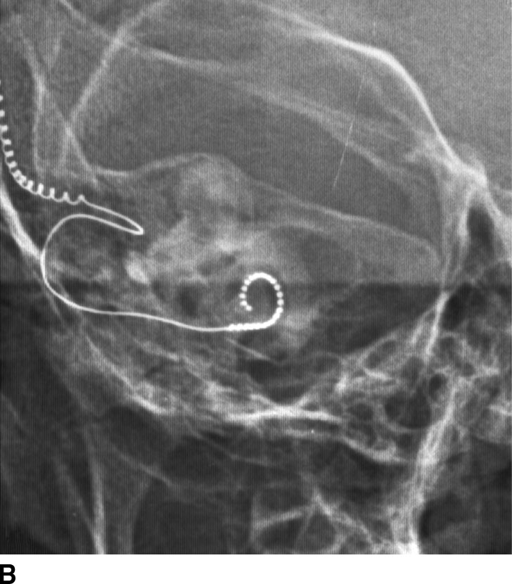
FIG. 1.1 Evaluation of cochlear implants with skull radiographs. A: AP view demonstrates bilateral cochlear implants in place, with receiver/stimulator overlying the lateral calvarium (white arrow) and electrode array overlying the region of the cochlea (black arrow). B: Magnified view of the right temporal bone demonstrates the normal curvature of the electrode array within the first turn of the cochlea.

Computed Tomography

CT uses ionizing radiation and a ring of detectors surrounding the subject to generate cross-sectional images of the brain (1). By moving a patient through a rotating ring of x-ray sources and corresponding detectors, tissue density within a specific voxel can be calculated using a mathematical analysis known as projection reconstruction. The computer detects an absorption value for each voxel within a cross-sectional slice. State-of-the-art multislice machines scan exceptionally fast with high spatial resolution. CT was one of the first reliable methods to visualize brain tissue and pathology in vivo and is still widely used today because of its relative low cost, widespread accessibility, and rapid acquisition time. CT scanning also allows for excellent delineation of bone and can often be a complementary way to study the brain, spine, and head and neck structures (Table 1.1).

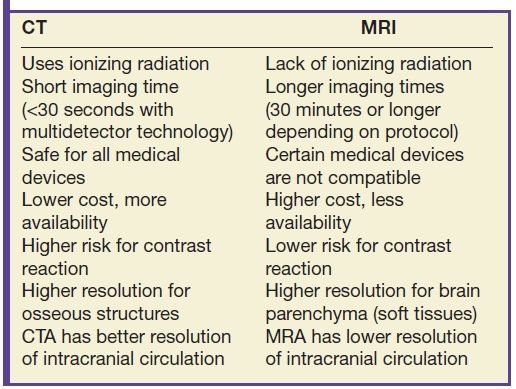
Table 1.1 COMPARISON OF CT AND MR IMAGING TECHNIQUES

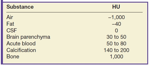
As mentioned, contrast on CT images is determined by detecting differences in x-ray absorption between tissue types. Attenuation is measured in Hounsfield units (HU) on a scale from −1,000 to +1,000, with 0 HU assigned to water attenuation, −1,000 to air attenuation, and +1,000 to bone attenuation. Familiarity with attenuation values for different tissue types and pathologies is crucial for image interpretation. Brain white matter and gray matter densities are in the 30- to 50-HU range. Fat is typically −40 to −100 HU. Acute hematoma ranges from 50 to 80 HU, and calcification/ossification is generally 150 HU or greater (Table 1.2). Attenuation measurements can vary based on technique, so comparisons across platforms should be done with care.

Table 1.2 HOUNSFIELD UNITS (HU) OF CENTRAL NERVOUS SYSTEM STRUCTURES ON CT

Reconstruction algorithm and window

Reconstruction algorithms are used to optimize observations within particular types of tissue. For example, a typical bone algorithm is used to accentuate the interface between the bone and other tissues and assess bone matrix to improve visualization of osseous lesions (Fig. 1.2).

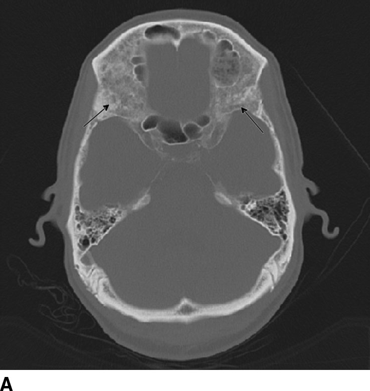
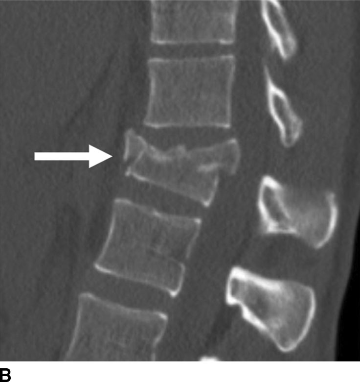
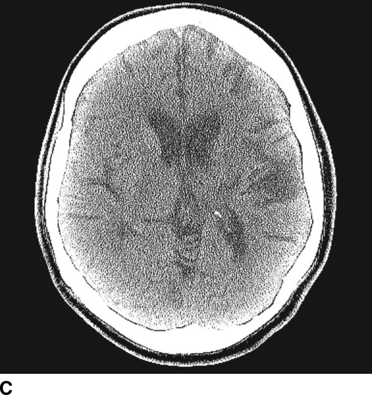
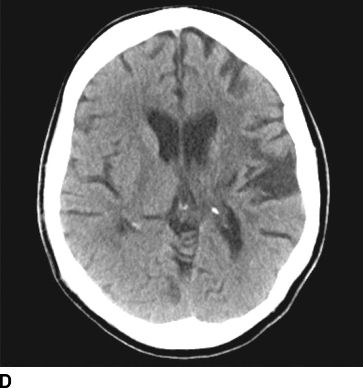
FIG. 1.2 Reconstruction algorithm. CT images reconstructed using bone algorithm and viewed with wide windows enhance details of osseous matrix. Seen here are typical lytic lesions of multiple myeloma (A) and compression fracture of a lumbar vertebra (B). Note that soft tissue is not well evaluated using a bone algorithm (C) but can be better assessed using an appropriate soft tissue algorithm (D).

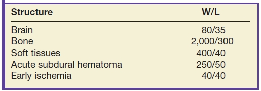
Separate from the reconstruction algorithm chosen, CT images can also be displayed using different window width and level settings. The window width is the range of HU displayed, and window level is the center point about which the range is displayed. Tissues within the window are assigned varying shades of gray. Tissues with HU out of the window will appear white and black, with higher and lower HU, respectively. Changing the viewing window endows CT with high contrast sensitivity: a window can be set to display very small as well as larger differences in tissue density. For example, the window can be optimized to visualize acute subdural hematomas as well as regions of acute infarction, commonly referred to as subdural and stroke windows (Fig. 1.3). Commonly used window and level (W/L) settings for different clinical situations are shown in Table 1.3.

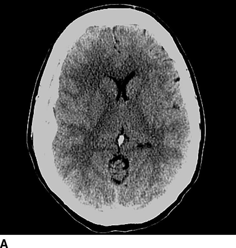
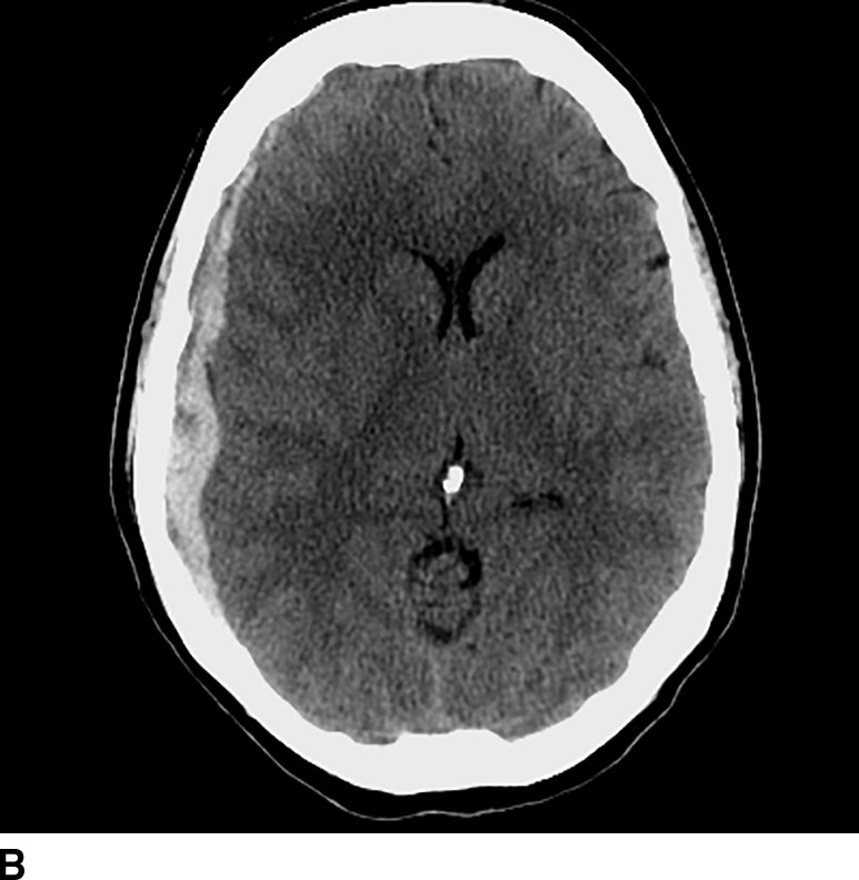
FIG. 1.3 Window and level Settings. The importance of selecting the appropriate window and level setting is to improve visualization of CNS pathology. Right convexity acute subdural hematoma is poorly seen on axial CT image using narrow “brain” windowing with window/level setting of 80/35 (A) but can be clearly appreciated using a subdural or intermediate window with window/level setting of 250/50 (B).

Table 1.3 COMMONLY USED WINDOW AND LEVEL (W/L) SETTINGS IN CT

Contrast-enhanced CT

While different types of tissues can exhibit contrast differences, it can be challenging to image and identify the interface between two adjacent tissues (e.g., brain parenchyma/tumor) or image soft tissues (e.g., clot) in contact with blood. In order to achieve higher levels of x-ray attenuation than those observed for biologic tissue, elements of higher atomic number (Z) are incorporated in a contrast agent molecule that can be administered intravenously. Iodine (Z = 63) has historically been the atom of choice for CT imaging applications (2). The most recent class of iodinated-based contrast agents is a dimer that consists of a molecule with two benzene rings (each with 3 iodine atoms) that does not dissociate in water (nonionic). For a given iodine concentration, the nonionic dimers have the lowest osmolality of all the contrast agents. At approximately 60% concentration by weight, these agents are iso-osmolar with plasma, which significantly decreases toxicity.

Even with improvements in their composition, risks associated with contrast agents have not been eliminated, and adverse reactions of varying degree continue to occur. Adverse reactions to intravenous contrast media are classified as idiosyncratic and nonidiosyncratic (3). Idiosyncratic reactions typically begin within 20 minutes of the contrast injection and are independent of the dose administered. Although these reactions have the same manifestations as do anaphylactic reactions, these are not true hypersensitivity reactions as IgE antibodies are not involved. Important implications of this difference include that a reaction can occur even the first time contrast is administered without prior sensitization, and the occurrence of a contrast reaction does not necessarily mean that it will occur again. Nonidiosyncratic reactions include vasovagal reactions, nephropathy, cardiovascular reactions, and extravasation.

Contrast is used in cranial CT to opacify blood vessels and to detect areas of breakdown of the blood–brain barrier. Intracranial masses, infectious and inflammatory, and vascular abnormalities should be evaluated with contrast. Aneurysms, arterial dissection, vessel occlusion, and arteriovenous malformations are well studied using CT angiography (CTA). CTA requires the rapid injection of approximately 50 to 125 mL of iodinated contrast material. High concentration contrast is recommended. Following contrast injection, imaging is done in the arterial phase and a 3D data set is acquired. Three-dimensional (3D) reconstructions of the data sets are especially helpful for better understanding the angioarchitecture of vascular lesions as well as their relation to the intracranial vasculature. Postprocessing software allows subtraction of the overlying, obscuring bony structures (4), which can be accomplished without a noncontrast mask with newer generation dual-energy CT scanners. Commonly used postprocessing techniques include maximal intensity projection (MIP) which projects the brightest pixels in the volume of interest for display, center-line reconstruction which follows the course of the vessel so that longer segments of the vessel may be assessed at the same time, and volume-rendered imaging in which it is easy to understand the three-dimensional relationship of the anatomy (Fig. 1.4).

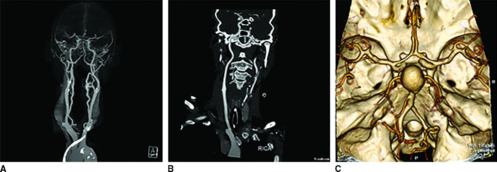
FIG. 1.4 CT angiography. Dual energy CT angiography allows single acquisition in the arterial phase and bone removal without applying a noncontrast mask (A). Center-line reconstruction of the right internal carotid artery (B) follows the artery through the skull base, an area typically difficult to assess. Volume-rendered image of the circle of Willis in a different patient (C) shows the irregular contour, so called “Murphy’s tit” along the posterior wall of a giant basilar tip aneurysm.

In addition to anatomical data, modern CT scanners can render physiologic data such as perfusion metrics (5). CT perfusion allows rapid qualitative and quantitative evaluation of cerebral perfusion by generating parametric maps of cerebral blood flow (CBF), cerebral blood volume (CBV), mean transit time (MTT), and time to peak (TTP). Perfusion imaging can be performed in a number of ways, but the most common technique in clinical practice involves an intravenous injection of contrast material that does not traverse the blood–brain barrier. Uninterrupted scanning at the same anatomic level, or cine scanning, performed at rapid rate for several seconds, allows for the visualization of the effect of the contrast agent as it traverses the vascular system (6).

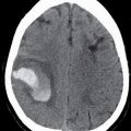
CT perfusion is useful for noninvasive assessment of cerebral ischemia, particularly in the assessment of acute stroke and aneurysmal subarachnoid hemorrhage (7). In the context of acute stroke, CT perfusion is a rapid technique that may help identify and quantify brain parenchyma at risk. The technique is based on the central volume principle (CBF = CBV/MTT) and employs deconvolution algorithms to produce perfusion maps. Most recently, newer deconvolution algorithms using the Bayesian estimation show promise in being more accurate than traditional delay-insensitive singular value decomposition algorithms that are widely available currently. In the setting of an acute infarction, areas of irreversibly infarcted tissue show matched areas of decreased CBF and CBV with increased MTT. This pattern suggests neuronal death with irreversible loss of function or core infarct (Fig. 1.5). On the other hand, regions of tissue that show decreased CBF with maintained CBV indicate potentially salvageable tissue or penumbra. Specific cut-offs have also been suggested for CBF to determine regions of core infarction. Although the exact clinical utility of CT perfusion in acute stroke and how best to reproducibly assess core infarct from penumbra remains controversial, the goal is to use noninvasive imaging to potentially extend the therapeutic window in specific patients.

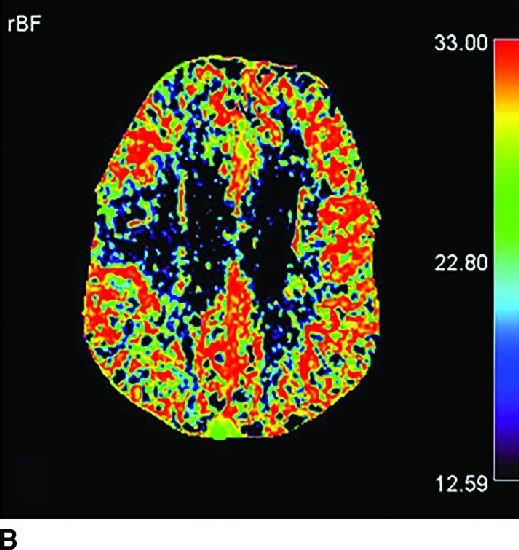
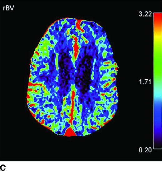
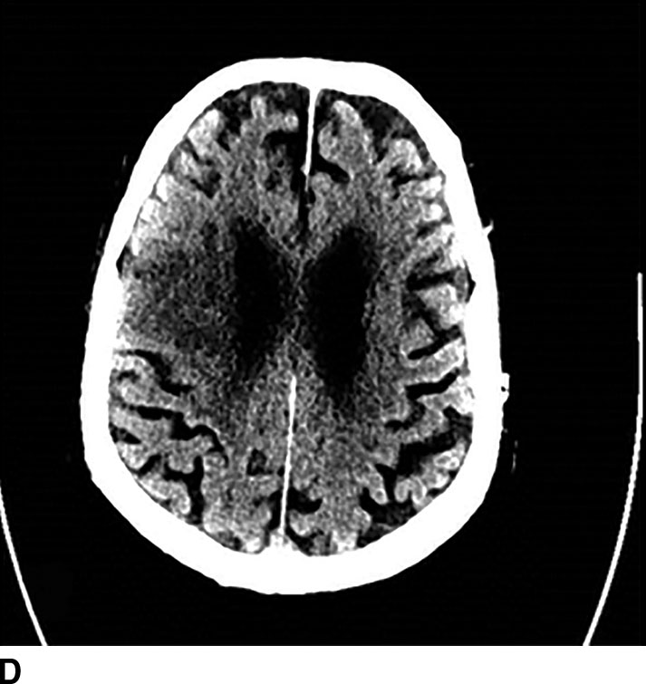
FIG. 1.5 CT perfusion: ischemic stroke. An 83-year old man presenting acutely with confusion and left-sided weakness. A: Admission noncontrast CT shows subtle hypodensity in the right corona radiata which is nonspecific (arrow). CBF map (B) and CVB map (C) obtained using Baysian estimation algorithm demonstrate a matched region involving right frontal cortex and corona radiata white matter of decreased blood flow and blood volume in keeping with an area of core infarction. Of note, increased pial collateral flow is seen in the ipsilateral hemisphere on CBV map. D: Follow-up noncontrast CT on day 2 after admission confirms a transcortical right frontal infarct in the region of the perfusion deficit.

Magnetic Resonance Imaging

In simplest terms, MRI creates images by exploiting the magnetic properties of protons in tissue by applying magnetic fields and exciting proton using radiofrequency (RF) pulses. Different types of tissues absorb and release radio wave energy at detectable and characteristic rates. Under usual conditions, protons in the body are aligned in random directions and therefore the body has no net magnetization. MRI scanners have a static magnetic field oriented along the longitudinal direction of the bore of the magnet. When placed in this field, some protons will align parallel to the direction of the main magnetic field, thus imparting a net magnetization to the tissue. MRI takes advantage of this magnetization to generate images.

A RF pulse applied at the resonant frequency excites protons from their alignment parallel to the main magnetic field. A 90-degree pulse, as is typically used in spin echo (SE) imaging, excites protons into a plane perpendicular to the main magnetic field. Protons also precess, or spin, in phase with each other yielding net transverse magnetization. Once the RF pulse is switched off, protons will return to an orientation parallel to the main magnetic field with the net longitudinal magnetization going back to its original value (longitudinal relaxation). Transverse magnetization decays as phase coherence dissipates. T1 relaxation rate measures the recovery rate of the longitudinal magnetization. T2 and T2* relaxation rates measure the decay rate of the transverse magnetization. Different relaxation rates in different tissues provide the bases for image contrast between tissue types. Such differences can be brought out using specifically designed pulse sequences (8). Advantages of MRI include excellent soft tissue resolution and lack of ionizing radiation to the patient (see Table 1.1).

The strong magnetic field within the MR scanner area requires specific safety measures to consider before performing or undergoing an MRI scan (9). The magnet may cause pacemakers, artificial limbs, and implanted medical devices that contain metal to malfunction or heat up during the exam. Ferromagnetic implants, such as cerebral aneurysm clips and skin staples are at risk for movement and dislodgement, burns, and induced electrical currents. Any loose metal object may cause damage or injury if it gets pulled toward the magnet. For these reasons, it is very important to cautiously screen patients before MR scanning and to assess which implants may be MRI compatible.

Conventional sequences

SE pulse sequences historically represent the standard sequences used in clinical neuroradiology, though many advances and improvements have now introduced a host of complex sequences that capitalize time efficiency, resolution, and tissue contrast. Two important parameters useful to be aware of in SE sequences are repetition time (TR), time between administered RF pulses, and echo time (TE), time between radio wave energy release and detection. SE T1-weighted images (T1WI) have relatively short TR and short TE, whereas T2-weighted images (T2WI) have long TR and long TE. Fat, proteinaceous material, methemoglobin, melanin, calcium, and paramagnetic contrast agents have short T1 relaxation time, appearing bright on T1WI, whereas fluid-heavy structures such as cysts, edema, and CSF are bright on T2WI. Conventional SE sequences have the disadvantage of being relatively slow sequences, and in clinical practice they have been replaced by gradient echo images and fast SE imaging (10).

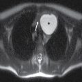
Inversion recovery (IR) pulse sequences are used to suppress signal from a specific type of tissue and have a variety of applications in MR imaging. In neuroimaging, the most common usage of IR is T2 fluid-attenuated inversion recovery (FLAIR), which eliminates signal from cerebrospinal fluid (CSF). T2 FLAIR sequences are useful to detect ependymal and periventricular abnormalities such as demyelinating plaques of multiple sclerosis (MS) (Fig. 1.6) (11). Another common IR sequence is short tau inversion recovery (STIR), in which signal from fat is suppressed and which is particularly useful in improving conspicuity of pathology in spine and head and neck imaging (Fig. 1.7) (12).

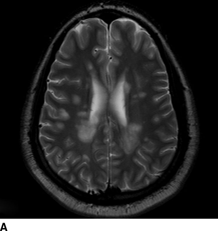
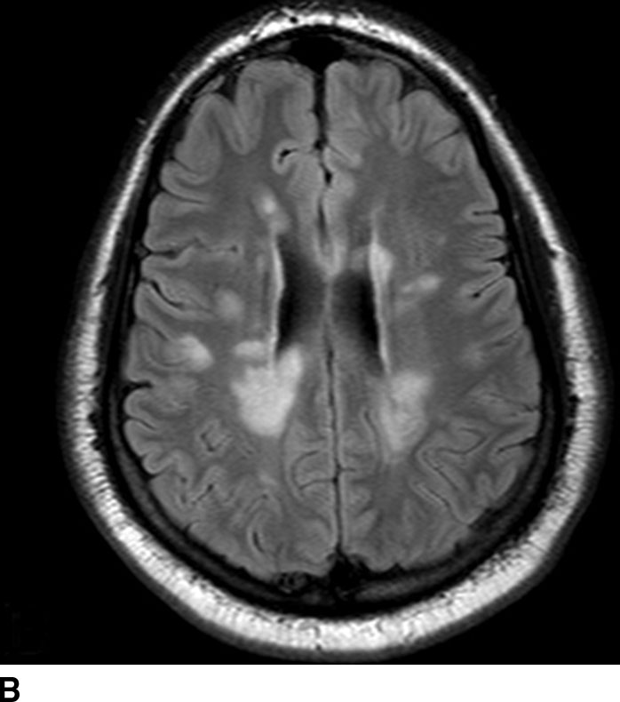
FIG. 1.6 Multiple sclerosis. Axial T2-weighted (A) and T2 FLAIR (B) images at the level of the lateral ventricles demonstrate periventricular areas of increased signal typical of the Dawson fingers of MS. T2 FLAIR images show these lesions to best advantage by nulling fluid signal in the CSF.

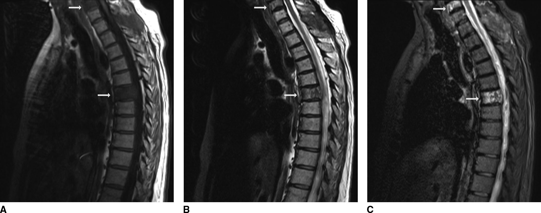
FIG. 1.7 Short tau inversion recovery (STIR): osseous metastatic disease. A 56-year-old female with a history of colon cancer presenting with back pain. There is abnormal signal on T1 (A), T2 (B), and STIR (C) images in the C6 and T6 vertebra (arrows) as well as in the T1 spinous process, most evident on STIR images, consistent with osseous metastases.

Gradient-recalled echo sequences

In gradient-recalled echo (GRE) sequences, instead of RF pulses, multiple gradients are used to phase and rephase the transverse magnetization. GRE sequences have the advantage of not being dependent on intrinsic T2 relaxation, and the dephasing and rephrasing gradients may be applied in quick succession, thereby allowing fast imaging. Often the initial RF pulse applied only partly flips the net magnetization vector into the transverse plane (13). GRE sequences are sensitive to magnetic field inhomegeneity secondary to magnetic susceptibility differences between tissues. This feature of GRE sequences is exploited for the detection of hemorrhage. The technique is useful for detecting blood products, iron deposition, and calcification (Fig. 1.8). A more recently developed pulse sequence, susceptibility weighted imaging (SWI), uses a 3D GRE sequence and incorporates information regarding phase differences to further increase the sensitivity in detecting susceptibility effects (14). SWI has been shown to be even more sensitive to blood products than is standard T2* GRE (15).

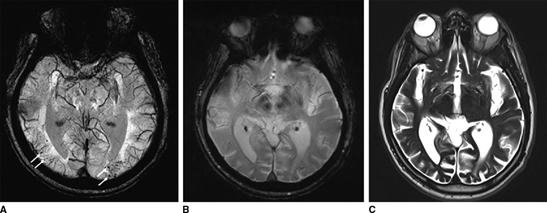
FIG. 1.8 Amyloid angiopathy. Susceptibility weighted imaging (SWI) (A), gradient echo (GRE) (B), and T2-weighted (C) images demonstrate multiple foci of abnormal susceptibility throughout the cortex typical of amyloid angiopathy. Notice how these areas are more conspicuous on SWI compared to GRE, and not so easily seen on the T2W image.

Contrast-enhanced MRI

Gadolinium is a paramagnetic agent with extremely short T1 relaxation time and can be used in TIWI. Because shortening of T1 leads to higher signal intensity on T1WI, areas of gadolinium accumulation will appear bright. As a free soluble aqueous ion, gadolinium is somewhat toxic, but is generally regarded as safe when administered as a chelated compound. In normal conditions, gadolinium does not cross the blood–brain barrier, and therefore contrast is usually absent in the brain. However, a few commonly visualized intracerebral structures do not have a blood–brain barrier. Thus, there is strong enhancement in the pituitary gland, the infundibulum, and the pineal gland following gadolinium contrast administration. Also, the mucosal surfaces of the nasopharynx and sinuses, slowly flowing blood, and the retinal choroid all show prominent contrast enhancement after the administration of MR contrast agent (16).

Gadolinium enhancement indicates regions of breakdown of the blood–brain barrier as gadolinium is bound to a chelating agent and the complex is a relatively large molecule that does not cross the blood–brain barrier under normal conditions. Thus, it can be very effective to detect areas of abnormality with respect to the blood–brain barrier including primary and secondary brain neoplasms (Fig. 1.9), infectious and inflammatory diseases of the central nervous system, as well as meningeal pathology (17–19).

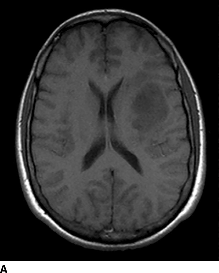
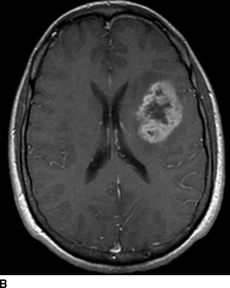
FIG. 1.9 Gadolinium-enhanced MRI: glioblastoma multiforme. T1WI before (A) and after (B) administration of intravenous gadolinium demonstrate peripherally enhancing left frontal lobe mass, pathologically proven to be glioblastoma multiforme. Contrast enhancement is consistent with areas of breakdown of the blood–brain barrier. Pre-contrast images should always be checked for intrinsic T1 shortening which can mimic enhancement such as from subacute blood products.

Only gold members can continue reading. Log In or Register to continue