Computer-Aided Image Analysis for Vertebral Anatomy on X-Ray CT Images

Fig. 7.1

New screening pathway via dental clinics with CAD system (adapted from [17])

Turning now to the topic of vertebral fracture, its risk is currently estimated on the basis of lumbar vertebral BMD in clinical practice. However, vertebral fractures can occur even when the BMD does not reach the osteoporotic threshold. There are some research findings on the vertebral fractures. For example, the compressive strength of vertebrae is determined not only by their bone density but also by their dimensions [18]. Reduced spinal sagittal curvature is an independent risk factor [19]. In spite of such discoveries, little is known about the role of vertebrae in fracture risk to date. It is likely that the sophisticated knowledge on normal vertebral anatomy is essential to understand the vertebral fracture risk.

Multi-detector row computed tomography (MDCT) scanning is widely used in clinical practice. It permits the acquisition of thin sections with isotropic voxel sizes. An example of body X-ray CT image is shown in Fig. 7.2. We see from Fig. 7.2 that human bone structures are radiologically visualized under high resolution. Namely, we can achieve the quantitative analysis of the vertebral anatomy such as volumetric BMD (vBMD), geometry, and alignment with high accuracy and precision from the same dataset by using the MDCT scanning. The problem is that such analysis takes a lot of time and effort. It is likely that computer-based image analysis is a key technology to overcome the above problem.

Fig. 7.2

An example of the body X-ray CT image

Here we present our latest studies of the computer-aided image analysis for vertebral anatomy by using the MDCT scanning. The second section describes a “Computer-Aided Analysis of vBMD at Trabecular Bones in Thoracic and Lumbar Vertebrae.” Computer-based quantification of vertebral body geometry is described in the third section. The findings of our studies and follow-up prospects are summarized in the section “Summary.”

Computer-Aided Analysis of vBMD at Trabecular Bones in Thoracic and Lumbar Vertebrae

The aims of this section were to investigate segmental variations in vBMD of thoracic and lumbar vertebral bodies and to show specific differences according to age and gender. First, a computer-assisted scheme to determine the volume of interest (VOI) at vertebrae was designed. And then, a large number of CT data set was employed to estimate the vBMD. On the basis of those results, we attempted to answer two key questions to improve our understanding of bone fragility: (1) Is there any vertebral level-dependent vBMD change? (2) Does the vBMD differ according to gender? This section summarized the publications in [20, 21] and it was beyond the scope of this section to discuss the clinical aspects.

Materials and Methods

Study Subjects

The study sample consisted of the first 1,750 enrolled Japanese men and women with CT images from 2002 to 2006, scanned for the purpose of examinations of various organs and tissues. The CT images included all thoracic and lumbar vertebrae [LightSpeed Ultra, GE Yokogawa Medical Systems Ltd, Tokyo, Japan] and were scanned for each subject using standard settings (120 kV, Auto mAs, 1.25 mm-thick slice, pitch = 0.49–0.88 mm) routinely used clinically. Slice intervals were modified to the same value as the pitch using sinc interpolation to keep each voxel in an isotropic size in 3-D.

Of the 1,750 individuals with CT data available, 719 were excluded because of normal variants, bone pathology, vertebral fractures, or reasons other than mild degenerative changes at vertebrae, as confirmed by radiologists or anatomic experts. The study subjects consisted, therefore, of 1,031 individuals: 490 men and 541 women. The study subjects were then subdivided into five age categories (≦40, 41–50, 51–60, 61–70, ≧71) in order to observe age differences. Low vBMD was measured in the front and central regions at the lumbar vertebrae in [22]. For this reason, the vBMD of trabecular bones at the central region of the vertebral body was decided as the typical site.

Computer-Assisted VOI Decision

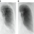
Each VOI from the first thoracic vertebra (T1) to the first sacral vertebra (S1) was determined as follows (Fig. 7.3).

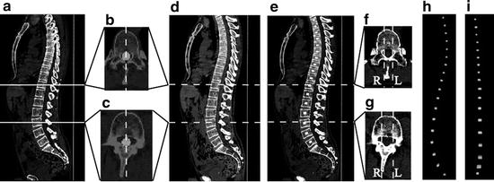
Fig. 7.3

Computer-assisted VOI decision. (a) One slice of sagittal section on CT images. (b, c) One slice of axial-sections of T11 and L3 on CT images, respectively (White circle denotes a segmented spinal canal). (d) Sagittal median plane image of the spine. (e) The VOI inputting on the sagittal median plane image of spine. (f, g) Input examples of the range of the right and left at T11 and L3 (White dash lines show the border of the VOI). (h, i) 3-D view of the inputted VOIs from the lateral and anterior sides, respectively (modified from [21])

The spinal canal regions were segmented based on the CT number and skeletal structures [23].

The central locations of the right and left sides of the spinal canal in each axial section were calculated, and a sagittal sectional image based on the center line of the spinal canal was generated. We defined the generated image as a sagittal median plane image of the spine. Figure 7.3b, c indicate the segmented spinal canal in one slice of axial sections of T11 and the third lumbar vertebra (L3), respectively (white circle denotes the segmented spinal canal). Figure 7.3d shows an example of the sagittal median plane image of the spine. Although there is no guarantee that the vertebral bodies of T1–S1 can be seen in only one slice of the sagittal sections of the original CT image (see Fig. 7.3a), T1–S1 can always be seen in the sagittal median plane image of the spine (see Fig. 7.3d).

The VOIs of T1–S1 were manually inputted on the sagittal median plane image of the spine. Inputted VOIs are shown by the white regions in Fig. 7.3e.

Axial sectional images of the original CT image corresponding to the center of each vertebra were referenced, and then we determined the right and left range of the VOIs. Input examples of the range of the right and left at T11 and L3 are shown in Fig. 7.3f, g.

Each VOI inputted at the process 3 was extended to the range inputted at the process 4. Examples of the VOIs obtained by the above method are shown in Fig. 7.3h, i. They show a 3-D view of the inputted VOI from the lateral and anterior sides, respectively. The 3-D volumetric VOI can be checked from their figures.

Estimation of vBMD

It is impossible to measure BMD using the established method proposed by Cann and Genant [24] (e.g., QCT) because the purpose of our CT data was not the diagnosis of osteoporosis. Instead of using “traditional” QCT, we fixed the standard phantom (B-MAS 200, Kyoto Kagaku, Kyoto, Japan) under the human body phantom, and took exposed it to the same radiation dose as that used in diagnosis in order to calibrate the CT Hounsfield units to equivalent bone mineral concentrations. The standard phantom contained calibration cells of 0, 50, 100, 150, and 200 mg/cm³ with equivalent concentrations of calcium hydroxyapatite. As a result, we estimated the vBMD as follows:

$\mathrm{vBMD}\left[\mathrm{mg}/{\mathrm{cm}}^3\right]=\left(\mathrm{CT}\ \mathrm{number}\left[\mathrm{HU}\right]-3.55\right)/1.13.$

(7.1)

Therefore, the mean CT number of the VOI determined in “Computer-Assisted VOI Decision” was computed. And then, the vBMD was estimated by using the calibration curve (i.e., Eq. 7.1).

Our New Findings on the Vertebral Trabecular vBMD

Vertebral Level-Dependent vBMD Change

The graph in Fig. 7.4 illustrates the vertebral level-dependent vBMD change in women between the ages of 51 and 60. We see from Fig. 7.4 that the vertebral level-dependent vBMD change is found and L3 has the lowest vBMD. Regardless of age and gender, similar level-dependent change was found in this study.

Fig. 7.4

Vertebral level-dependent vBMD change (modified from [21])

Gender-Dependent vBMD Change

The graphs in Fig. 7.5 illustrate the gender-dependent vBMD change in the ages of 40 and 61–70. We see from Fig. 7.5 that gender-dependent vBMD change is found. Regardless of vertebral level, women in the ages of 40 had the highest vBMD. However, the women’s vBMDs rapidly deteriorated with aging.

Fig. 7.5

Gender-dependent vBMD change (modified from [21])

Deterioration of vBMD with Aging

Tukey multiple comparison test was used to understand the deterioration of vBMD with aging. Significant difference was defined as p < 0.05. Correlation value of the vBMDs between 41–50 years and other age categories is represented in Fig. 7.6. As for comparison with 51–60 years, a glance at Fig. 7.6a will reveal that the significant differences are found in all vertebral levels in women. In contrast, the significant differences are not found in all vertebral levels in men (see Fig. 7.6b). As for comparison with 61–70 years in men, the significant differences are found in the vertebral levels from T10 to L5 (see Fig. 7.6c). As for comparison with 71 years in men, the significant differences are found in all vertebral levels. Therefore, it is suggested that the deterioration of the vBMDs is similar in all vertebral levels in women, whereas it is faster at T11–L5 levels than at T1–T10 levels in men. It should be noted that its cause is not clear and further studies are required.

Fig. 7.6

Correlation value of the vBMDs between 41 and 50 years and other age categories by using Tukey multiple comparison test. Significant difference was defined as under 0.05 (as shown in filled circle) (a) Comparison with 51–60 years. (b) Comparison with 61–70 years. (c) Comparison with ≧71 years (modified from [21])

Computer-Based Quantification of Vertebral Body Geometry

We described in this section the computer-based quantification of the vertebral body geometry. For gaining a better understanding of bone quality, a great deal of attention has been paid to vertebral geometry in anatomy [18]. In order to accelerate such basic investigation, it may be helpful to develop a computer-assisted scheme for analyzing the vertebral geometry on body CT images.

It is thought that to design a sophisticated scheme for the localization of individual vertebral bodies would be helpful first to design a computer-assisted scheme to analyze the vertebral geometry. Although extraction of intervertebral discs (or end plates) is one of the effective approaches, missing an intervertebral disc leads to failure in the localization of vertebral bodies. Pattern matching or a registration-based approach can localize the vertebral bodies without extracting intervertebral discs. However, variations in the individual’s posture during CT scans or individual differences in spinal curvature may contribute to the performance deterioration of such an approach. In terms of implicit anatomic knowledge, ribs and thoracic vertebrae are contiguous bones. For this reason, we assume that the detection of individual ribs contributes to the scheme’s improved performance for the localization of individual vertebral bodies.

Our new scheme was designed to have the following key steps: (1) re-forming CT images on the basis of the center line of the spinal canal to visually remove the spinal curvature, (2) using the information on the relative position between ribs and vertebral bodies, (3) the construction of a simple model (reference pattern) on the basis of the contour of the vertebral bodies on CT sections, (4) the localization of individual vertebral bodies by using a template matching technique, and (5) quantification of the vertebral body width, depth, cross-sectional area (CSA), and trabecular vBMD. This section summarized the publications in [25–27].

Computerized Scheme to Quantify the Vertebral Geometry

Overview of the Scheme

The proposed scheme is outlined in Fig. 7.7. It consists of the learning and test phases. The image re-formation technique, which is done on the basis of the detection/extraction of bone parts, is applied in both phases. The localization of vertebral bodies is carried out using a template matching technique. Afterward, the localization results are used to quantify the vertebral geometry. Each process is described below.

Fig. 7.7

Process flow of our scheme that quantifies the vertebral geometry (spinal canal: SC, spinous processes: SP) (modified from [25, 26])

Image Re-Formation

At the beginning of the image re-formation technique, bone extraction and detection of the center line of the spinal canal, the tips of the spinous processes, and the ribs (boundary with vertebrae) are attempted. Examples of these extractions and detections are shown in Fig. 7.8.

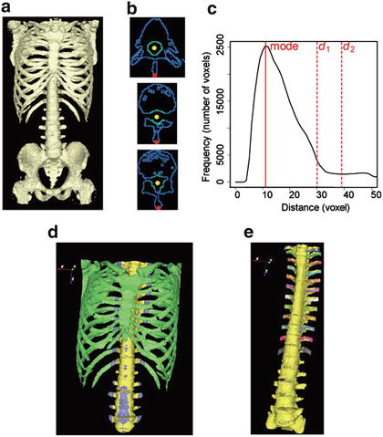
Fig. 7.8

Examples of bone parts detection/extraction in one case. (a) Surface view of bone voxels. (b) Three axial section views of bone voxels (top to bottom: T6, T11, and L3). Yellow and red circles denote centroids of the spinal canal and tips of spinous processes, respectively, and standard voxels and other bone voxels are indicated in green and blue, respectively. (c) The histogram of the distance map. d ₁ and d ₂ denote distance thresholds for dividing bone labels. (d) Surface view of bone voxels divided into three labels (spine_label, boundary_label, and the_others_label are indicated in yellow, blue, and green, respectively). (e) Surface view of bone voxels identified right and left ribs in each level (spine and ribs in each level are shown in yellow and the other colors, respectively) (adapted from [25])

CT numbers with bone voxels are higher than those of other internal organs. CT number thresholding or the region-growing method is used to extract bone voxels [28]. Figure 7.8a shows an example of extraction of bone voxels.

We can observe the spinal canal as a cave inside the spine. For that reason, the centroid of the cave on the Jacoby line (an upper boundary slice with a false pelvis) is determined. After that, it is tracked in the craniocaudal direction [29].

Spinous processes can be observed as tips of bone behind the spinal canal. Therefore, these tips of bone are detected on axial sections excluding the tail sections from the Jacoby line. Detection of the center line of the spinal canal and tips of spinous processes in three axial sections (from top to bottom: T6, T11, and L3) are shown in Fig. 7.8b. In these sections, yellow and red circles denote centroids of the spinal canal and tips of spinous processes, respectively.

Ribs are contiguous bones with the spine. In our scheme, ribs are detected on the basis of their distance from the spinal canal. The detailed process is as follows:

Bone voxels within r mm of the center line of the spinal canal are extracted as standard voxels. Extraction examples in three axial sections are illustrated in Fig. 7.8b. In these sections, standard voxels and other bone voxels are indicated with green and blue, respectively.

The distance map from standard voxels is generated. The distance is calculated by the shortest path through the bone voxels.

The histogram of the distance map is generated, and its mode and a standard deviation are computed. While frequency values increase with increasing distance within the spine, they decrease with increasing distance at the ribs because they are thinner than the spine. Therefore, the following equations are defined for dividing three bone labels (spine_label, boundary_label, and the_others_label) using the distance map:

$0< spine\_ label\le {d}_1,$

(7.2)

${d}_1< boundary\_ label\le {d}_2,$

(7.3)

${d}_2< the\_ others\_ label,$

(7.4)

${d}_1= move\_ value+ standard\_ deviation\cdot {b}_1,$

(7.5)

and

${d}_2= move\_ value+ standard\_ deviation\cdot {b}_2,$

(7.6)

where d ₁ and d ₂ denote distance thresholds and b ₁ and b ₂ denote arbitrary variables. The histogram of the distance map and an example of the division into three bone labels are illustrated in Fig. 7.8c, d, respectively. In Fig. 7.8d, spine_label, boundary_label, and the_others_label are indicated in yellow, blue, and green, respectively. We can see the relation between distance map and bone labels in these figures.

Of the boundary labels, labels contiguous to both the spine_label and the_others_label are detected as rib_candidate_labels.

Of the rib_candidate_labels, 12 labels from the head are identified as the 1st–12th ribs. This identification is performed independently on the right and left sides. An example of 1st–12th ribs identification is demonstrated in Fig. 7.8e, in which the spine and the right and left ribs in each level are shown in yellow and the other colors, respectively.

To simplify the localization of vertebral bodies, CT images are re-formed on the basis of the spinal canal and spinous processes. The following three rules are applied to image re-formation.

Axial rotation is adjusted in each slice so that the line via the center line of the spinal canal and tips of the spinous processes (that is, the black dashed line shown in Fig. 7.9a) becomes the center in the sagittal direction.

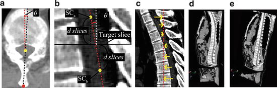
Fig. 7.9

CT images re-formation based on the spinal canal and spinous processes. (a) An axial section view of the spine. Yellow and red circles denote centroid of the spinal canal and the tip of spinous processes, respectively, and an axial rotation of this section is defined as the angle between the black dashed line via centroid of the spinal canal and the tip of spinous processes and red dashed line that indicates vertical line. (b) A sagittal section view of the spine. SC_a and SC_b denote centroid of the spinal canal on two axial sections. Sagittal rotation at a target slice is defined as the angle between the red dashed line via SC_a and SC_b and the white dashed line that indicates vertical line. (c) A sagittal section view of the spine. The translation is performed so that the center line of the spinal canal moves onto the straight line (red dashed line). (d) Section view of CT images. We can see the spinal curvature. (e

Only gold members can continue reading. Log In or Register to continue