Cortex Segmentation on Computed Tomography

Fig. 1

Kidney. (a) The kidney in one CT slice. (b) Iso-surface rendering [7]

The renal cortex, medulla, and pelvis are three basic compartments of kidneys. Only out-layer of the kidney is strictly defined as a renal cortex because renal columns are anatomically and functionally different from the cortex. Several previous researches treated renal cortex and column as homogeneous structures though they are anatomically different. However, only the out-layer of the kidney (i.e., renal cortex) needs to be quantified with volume and thickness in most clinical applications. For certain clinical studies, it is advisable to measure the renal cortex precisely.

The renal cortex segmentation is one of fundamental steps for renal cortical volume and thickness measurement, since the quantification of renal cortical volume and thickness plays an important role in renal function analysis. However, kidney and renal cortex segmentation is a challenging task. As shown in Fig. 1, the location of kidney in abdomen and its specific internal anatomical structures in CT images are visualized in one slice (see Fig. 1a), and the surface of different internal anatomical structures is also rendered (see Fig. 1b). Surrounding anatomical structures or organs, such as liver, spine, and muscles, are located beside the kidney. In addition,the boundaries with adjacent anatomical structures are weak. Image artifacts, noise, and various pathologies, such as cancers and nephrolithiasis, pose more challenges. The renal cortex and renal column are fused as one connected component, since they have similar intensity distributions. The renal cortex is a non-fully closed structure due to the renal pelvis [7]. Currently, the renal cortex segmentations used in many clinical situations rely on manual methods, which are subjective, tedious, time-consuming, and prone to errors. Hence, there is a strong need to develop a fully automatic and accurate kidney and renal cortex segmentation.

Imaging Protocol

Computed tomography (CT) imaging, magnetic resonance imaging (MRI), and ultrasound (US) imaging are widely used for kidney examination and kidney diseases diagnosis because essential anatomical information, including kidney morphology and kidney ducts, can be readily obtained [8–11].

Computed tomography (CT) scan is a noninvasive diagnostic imaging modality that uses a combination of X-rays and computer technology to produce detailed cross-sectional images (often called slices) of the body. A beam of X-rays is aimed at one part of body, for instance, abdomen, which needs to be checked. Energy of beam attenuates as it passes through skin, bone, muscle, and other tissue. These variations can be detected by a two-dimensional monitor behind the body part. The X-ray beam moves in a circle around the body inside CT gantry. After the projection is accomplished in one direction, the X-ray signals are transmitted to a computer in order to reconstruct a series of slices.

CT imaging of the kidneys is useful in the examination of one or both of the kidneys to detect conditions obstructive conditions, such as kidney stones, congenital anomalies, polycystic kidney disease, accumulation of fluid around the kidneys, and the location of abscesses. The CT images can also present precise information about the size, shape, and position of a tumor. It is also useful in checking to see whether a cancer has spread to organs and tissues beyond the kidney and can help find enlarged lymph nodes that might contain cancer.

Although high resolution CT has taken the largest leap, MRI is also an imaging technique used primarily in medical settings to produce 3D high-quality morphologic images of the inside of the human body in the evaluation of renal abnormalities. MRI modality can be applicable to children and pregnant women since it does not lead to radiation exposure, compared to CT modality. MRI uses a powerful magnetic field, radio waves, and a computer to produce detailed pictures of organs, soft tissues, bone, and virtually all other internal body structures. The energy from the radio waves is absorbed and then released in a pattern formed by the type of body tissue and by certain diseases. A computer translates the pattern into a very detailed image of parts of the body. A contrast material called gadolinium is often injected into a vein before the scan to better see details. This contrast material cannot be used in people on dialysis, because in those people it could cause a severe side effect called nephrogenic systemic fibrosis. Additionally, dynamic contrast-enhanced MRI is often used for renal lesion characterization. The multiphase 3D volume interpolation is performed as multiple breath-hold sequences before and at timed intervals after intravenous bolus injection of a gadolinium-based contrast agent. It allows for more accurate computer-processed image subtraction and better degree of lesion enhancement with reproducible diaphragmatic excursion during breath-holds.

MRI still plays an important role in differentiating benign lesions versus malignant lesions of patients in renal imaging. MRI can achieve the similar accuracy as CT in detection and characterization of most renal lesions, including malignant renal lesions such as renal cell carcinomas, and benign renal lesions such as oncocytoma and angiomyolipoma. In addition, MRI has a high sensitivity in evaluating complicated cysts and early lymph node spread and can be used to analyze lesions with minimal amounts of fat or with intracellular fat. Functional MRI of the kidney has found broad clinical application. It can be used in the analyses of compromised renal function, severe contrast allergy. Attempts are being made to use MRI for imaging of renal function, including perfusion, glomerular filtration rate, and intra-renal oxygen measurement.

Ultrasound (US) imaging of kidney is also a noninvasive and painless modality used to obtain the size, shape, and location of the kidneys with no radiation exposure. This modality uses sound waves to create images of internal organs. A handheld transducer is utilized to send out ultrasonic sound waves at a frequency. The ultrasonic sound waves go through the skin and other body tissues to the organs and structures of the abdomen as the transducer is placed on the abdomen at certain locations and angles. The sound waves bounce off the tissues in the organs like an echo and return to the transducer. The transducer picks up the reflected waves, which are then converted into an image of the organs.

Ultrasound imaging can help determine if a kidney mass is solid or filled with fluid. Therefore, blood flow to the kidney can be assessed by using an additional mode of ultrasound technology during an ultrasound imaging. An ultrasound transducer with a Doppler probe is used to assess blood flow. By making the sound waves audible, the Doppler probe within the transducer evaluates the velocity and direction of blood flow in the vessel. The degree of loudness of the audible sound waves suggests the rate of blood flow within a blood vessel. Absence or faintness of these sounds may show an obstruction of blood flow. In addition, ultrasound imaging is suitable for detection and characterization of tumors, since the echo patterns produced by most kidney tumors are different from those of normal kidney tissue. Different echo patterns can distinguish some types of benign and malignant kidney tumors. This imaging modality can be used to guide a biopsy needle into the mass to obtain a sample if a kidney biopsy is needed.

General Frameworks

In computer vision and image analysis, image segmentation is a fundamental and challenging problem. In medical image processing, several challenges still remain in spite of several decades of research and many key technological advances. The medical image segmentation methods may be classified into three frameworks: image-based [12–23], model-based [24–32], and hybrid methods [33–40]. Image-based methods perform segmentation based only on information available in the image; these include thresholding, region growing [12], morphological operations [13], active contours [14, 15], level sets [16], live wire [17], watershed [18], fuzzy connectedness [19, 20], and graph cut [21, 22]. These methods perform well on high-quality images. However, the results are not as good when the image quality is inferior or boundary information is missing. In recent years, there has been an increasing interest in model-based segmentation methods. One advantage of these methods is that, even when some object information is missing, such gaps can be filled by drawing upon the prior information present in the model. The model-based methods employ object population shape and appearance priors such as atlases [24, 25, 29, 30, 41], statistical active shape models [26, 42, 43], and statistical active appearance models (AAMs) [27, 31, 32]. As such, hybrid methods that form a combination of two or more approaches are emerging as powerful segmentation tools, where their superior performances and robustness over each of the components are beginning to be well demonstrated [33–40].

Typically, image information, such as, the spatial information and intensity, were used for kidney and renal cortex segmentation with image-based methods. Boykov and colleagues [44] developed a temporal Markov model to describe the time intensity curves for each pixel and used the min-cut/max-flow algorithm for kidney segmentation [45]. Sun et al. [46] presented an integrated image registration algorithm to segment renal cortex in MR images. Zöllner et al. [47] applied automated image analysis methods in the assessment of human kidney perfusion based on 3D dynamic contrast-enhanced MRI data. Song et al. [48] combined spatial anatomical structures with temporal dynamics for dynamic MR images kidney segmentation.

Another type is model-based segmentation framework. Freiman et al. [49] proposed a nonparametric model constraint graph min-cut/max-flow approach for automatic kidney segmentation in CT images. Tsagaan et al. [50] integrated the gray level appearance of the target and statistical information of the shape into NURBS surface-based deformable model to automatically segment kidneys from abdominal 3D CT images. Touhami et al. [51] proposed a statistical method for fully automatic kidneys segmentation. They used spatial and gray-levels prior models by using a set of training images.

Several prior investigations have addressed the kidney and renal cortex segmentation on hybrid methods. In order to automatically segment kidney parenchyma in MR datasets, Gloger et al. [52] first applied a multistep refinement approach to improve the quality of the probability map, and then an extended prior shape level set segmentation method was used on the refined probability maps and combined several relevant kidney parenchyma features. Lin et al. [53] proposed a two-step fully automatic kidney parenchyma 3D segmentation technique in MR datasets to segment kidney in CT images. Xie et al. [54] introduced a texture and shape priors-based method in ultrasound images. Li et al. [55] presented a graph construction-based optimal graph search method for renal cortex segmentation on CT images. Li et al. [7] also presented an automatic renal cortex segmentation approach by the combination of the implicit shape registration and novel multiple surfaces graph search.

In Fig. 2, the kidney cortex framework is divided into two phases: training and segmentation. In the first phase, landmarking is used to annotate kidney’ shape, an AAM is built, and then the live wire and graph cuts parameters are trained. The second phase consists of two main steps: initialization and delineation. In the initialization step, a pseudo 3D initialization strategy is applied such that the contour of the kidney is obtained slice by slice via a multi-object AAM method. A refinement operation may be done subsequently to correct improperly initialized slices. We employ the pseudo-3D initialization strategy motivated by its efficiency and ability to combine. The strategy is much faster while achieved a similar performance compared to a full 3D initialization method. Additionally, it is difficult to integrate AAM into live wire in 3D. In the delineation step, we compute the graph cuts cost based on the shape information generated from the oriented active appearance model (OAAM) initialization step. The kidney is delineated using the iterative graph cut OAAM method. After getting the kidney contour, we employ morphological operations to obtain the initial cortex shape. Finally, the shape constrained iterative graph cut OAAM method is applied once more to segment the renal cortex. The details of each step are described in the following sections.

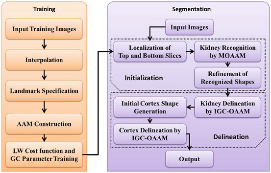
Fig. 2

The framework of the proposed method (AAM active appearance model, LW live wire, GC graph cuts, MOAAM multi-object active appearance model, IGC–OAAM iterative graph cut-oriented active appearance model)

Kidney Modeling

The literature is rich with kidney modeling approaches. To segment 3D kidneys in CT images, more detailed active shape models were generated and did not need to explicit or parametric formulations of the problem. The active shape model was quickly updated with additional prior knowledge. In addition, the crucial correspondence problem is solved by nonrigid image registration [56]. Tsagaan et al. [50] presented a deformable model-based approach for automated segmentation of kidneys from 3D abdominal CT images. Spatial and gray-levels kidney prior models were used according to a set of training images [51]. In the paper of Lin et al. [53] he presented a directional model-based approach for computer-aided kidney segmentation of CT images. Xie et al. [54] introduced a texture and shape priors-based method in ultrasound images. In the framework shown in Fig. 2, the top and bottom slices of each kidney are first manually selected before the AAM is constructed. Then linear interpolation is executed to generate the same number of slices for the kidney in every training image, in order to establish anatomical correspondences. 2D OAAMs are then built for each slice level from the images in the training set. The cost function of live wire and parameters of graph cuts are also obtained in this phase.

Landmark Specification

A 3D shape of kidney is represented as a stack of 2D contours and also manually annotated slice by slice. Because of its simplicity, generality, and efficiency, manual landmarking is still in use in clinical research, although semiautomatic or automatic methods are also available for annotating kidneys. Therefore, manual landmarking is applied to annotate kidney’s shape. Prominent landmarks on each shape are identified by trained operators and also visualized on slices.

The equally spaced landmarking method [57] was assessed, in order to demonstrate that there is a strong correlation between the shapes annotated by the manual and semiautomated landmarking approaches. In practice, the shape of an object can be represented by a finite subset of a sufficient number of its points; hence the shape of a kidney is treated as an infinite point set. Then, different numbers of landmarks are used for different kidneys from different medical images based on their size. Numerous researches have been done for the analysis of effects of distribution of landmarks on model building and segmentation results; these experiments consequently were omitted while manual landmarking was validated by the equally spaced labeling method.

Active Appearance Model Construction

The standard AAM [31, 32] method is applied to build the model after the landmarks are specified. Shape and texture information are integrated into the model. Suppose M _jdenotes the AAM for slice level j and the number of slice levels is n, then the complete AAM M can be represented as M = (M ₁,M ₂, …,M _n).

Although a pseudo 3D initialization strategy is applied, the fully 3D AAM denoted M _3D is also constructed by using the method in [58]. This 3D model is used to only provide the delineation constraints as explained later.

Live Wire Cost Function and Graph Cuts Parameter Training

An oriented boundary cost function is designed for a kidney included in the model M as per the Live Wire method [16]. Following the original terminology and notation in [16], a boundary element, bel for short, is defined as an oriented edge between two pixels with values 1 and 0. A bel is represented as an ordered pair (p,q) of four-adjacent pixels where p is inside the kidney (pixel value is 1) and q is outside (pixel value is 0) for a given image slice I, as shown in Fig. 3. Every pixel edge of I is considered as constituting two potential bels(p,q) and (q,p) and possibly assign different cost values to them. The features assigned to each bel are used to represent the likelihood of the bel that belongs to the boundary of a particular object of interest.

Fig. 3

The four possible situations that a boundary element is an oriented pixel edge. The inside of the boundary is to the left of the bel and the outside is to the right of the bel

The cost c(l) associated with bel l is a linear combination of the costs assigned to its features,

$c(l)=\frac{{\displaystyle \sum_{i=1}^{nf}{w}_i{c}_{\mathrm{f}}\left({f}_i(l)\right)}}{{\displaystyle \sum_{i=1}^{nf}{w}_i}}$

(1)

where, nf denotes the number of features, w _idenotes a positive constant indicating the emphasis given to feature f _i, and c _f denotes the function to convert feature values f _i(l) at l to cost values c _f(f _i(l)). f _imay represent features such as intensity on the immediate interior of the boundary, intensity on the immediate exterior of the boundary, and gradient magnitude at the center of the bel in [16]. Different f _imay be combined, which depends on the intensity characteristics of the object of interest. As suggested in [16], c _f is chosen as an inverted Gaussian function, and all selected features are combined with uniform weights w _i. We employ the feature of live wire to define the best-oriented path between any two-landmark points (x _kand x _k+1) as a sequence of bels with minimal total cost:

$\kappa \left({x}_k,{x}_{k+1}\right)={\displaystyle \sum_{i=1}^hc\left({l}_i\right)}$

(2)

where h is the number of bels in the best-oriented path (l ₁,l ₂, …,l _h). The total cost structure K(x) associated with all the landmarks may be formulated as

$K(x)={\displaystyle \sum_{k=1}^m\kappa \left({x}_k,{x}_{k+1}\right)}$

(3)

where m denotes the number of landmarks for the object of interest, and we assume that the contour is closed, i.e., x _m+1 = x ₁. In other words, K(x) represents the sum of the costs associated with the best-oriented paths between all m pairs of successive landmarks of shape instance x. The parameters of K(x) for each object shape x are obtained automatically as described in [16] by using the training images.

For the sake of continuity, the description of how the parameters of graph cuts are estimated is given in section “Kidney and Renal Cortex Segmentation” where the graph cuts algorithm is described.

Kidney Localization

The initialization step plays a critical role in the segmentation of kidney and renal cortex framework. The subsequent segmentation tends to have higher accuracy when initial model is localized in the region closer to kidney. To segment the kidneys in dynamic contrast-enhanced MRI, graph cut method was used based on min-cut/max-flow algorithm [45], where the localization was accomplished by painting foreground seed points and background seed points on some slices [44]. Tsagaan et al. [50] presented automated positioning method of an initial model for automated segmentation of kidneys from abdominal 3D CT images. The candidate kidney region was detected according to the statistical geometric location of kidney within the abdomen in [53]. This method can be applied to images of different sizes since they used the relative distance of the kidney region to the spine. In the work of Li et al. [55], the coarse pre-segmentation was firstly obtained by using Amira. Recently, the whole kidney was coarsely initialized using an implicit shape registration method in [7].

In this framework, the initialization method provides the shape constraints to the subsequent graph cuts delineation step and makes the delineation fully automatic. The developed initialization method is divided into three main steps. First, a slice localization method is employed to identify the top and bottom slices of the kidneys. A linear interpolation is then utilized to generate the same number of slices for the given image of a subject as in the model. The kidneys are recognized slice by slice via the OAAM method. A multi-object strategy [59] is applied to help with kidney recognition. Even if just one kidney is to be segmented, other organs can also be included in the model to provide context and constraints. Finally, a refinement approach is used to adjust the initialization result.

Localization of Top and Bottom Slices

There are several recent researches related to slice localization. Haas et al. [40] created a navigation table with eight landmarks, which were identified in various ways. By using probabilistic boosting tree and Haar features, Seifert et al. [42] developed a method to detect invariant slices and single point landmarks in full body scans. Emrich et al. [60] introduced a CT slice localization approach by using k-nearest neighbor instance-based regression. The target of slice localization is to identify the top and bottom slices of the organ in our framework. The model can be utilized to locate slices, since the model is already trained for each kidney slice. The proposed approach is based on the similarity of the slice to the OAAM.

The top slice model is used for each slice in the image based on the recognition method described in section “Kidney and Renal Cortex Segmentation,” in order to locate the top slice in a given image. Then the slice corresponding to maximal similarity or minimal distance is considered as the top slice of the kidney. Figure 4 shows the localization of the top slice in a CT image, where the distance value is computed from (5). The minimal value corresponds to the top slice of the left kidney. A similar method is applied to detect the bottom slice.

Fig. 4

Illustration of top slice recognition [61]. (a) A slice of the abdominal region. Cross point is the top slice of the left kidney. (b) The distance values of each slice to the top slice are plotted for the left kidney

Kidney Recognition by Multi-object Active Appearance Model

The kidney recognition method is based on the AAM. The root mean square difference between the appearance model instance and the target image is achieved in traditional AAM matching method for object recognition. It is more suitable for matching appearances than for the detailed segmentation of target images in this procedure (shown in Fig. 5b). The reason is that the AAM is optimized on global appearance; therefore, it is less sensitive to local structures and boundary information in this procedure. In contrast, the live wire detects the boundary very well [16], but it needs good initialization of landmarks and user interaction. Therefore, live wire is integrated into AAM, in order to combine their complementary strengths. In the new procedure, the landmarks needed in the live wire are provided by the AAM; meanwhile, the shape model of the AAM can be improved by live wire. The live wire is fully integrated into AAM in two aspects: First, the shape model of the AAM is improved based on the live lire method; second, the live wire boundary cost is integrated into cost computation during the AAM optimization process. As shown in Fig. 5c, the boundary detection is much improved with the proposed OAAM segmentation, compared to traditional AAM method (see Fig. 5b).

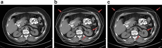
Fig. 5

Comparison of traditional active appearance model and oriented active appearance model segmentation [61]. (a) Original image. (b) Traditional active appearance model segmentation. (c) Oriented active appearance model segmentation

Refinement of the Shape Model in Active Appearance Model by Live Wire

First, a rough placement of the model is achieved by using the conventional AAM searching method. The shape is obtained from the shape model of the AAM, and then live wire is applied to update the landmarks using only the shape model and the pose (i.e., translation, rotation, and scale) parameters in [33], as shown in Fig. 6. The refined shape model is subsequently transformed back into the AAM. Meanwhile, AAM refinement is utilized to yield its own set of coefficients for shape and pose.

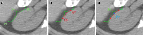
Fig. 6

The position of the landmarks [61]. (a) P ₁, P ₂, and P ₃ are three landmarks from active appearance model. (b) The middle point Q ₁ of the live wire segment between P ₁ and P ₂, and Q ₂ for P ₂ and P ₃ are obtained. (c) Landmark P ₂ is moved to the closest point P′₂ on the live wire segment from Q ₁ to Q ₂

Algorithm 1: Refine Active Appearance Model Shape Model Based on Live Wire

Input: The shape model x.
Output: Updated shape model x′ and new affine transformation t′.
Begin
For each triple P ₁, P ₂, and P ₃ of successive landmarks on x

1.

Delineate from P ₁ to P ₂ and P ₂ to P ₃ via Live Wire.

2.

Search the middle point Q ₁ and Q ₂ in the Live Wire segments obtained from P ₁ to P ₂ and from P ₂ to P ₃, respectively.

3.

Delineate from Q ₁ to Q ₂ via Live Wire.

4.

Search the point P′₂ on the Live Wire segment from Q ₁ to Q ₂ closest to P ₂, and update P ₂ to P′₂.
EndFor

5.

Transform the obtained shape x _rinto a new shape model instance x′ by aligning x _rto the mean shape $\overline{x}$ , in order to yield the new affine transformation t′.

6.

Apply the model constraints to the new shape model x′ so that the new shape is within the allowed shape-space.
End

Oriented Active Appearance Model Optimization

The boundary cost is not taken into consideration in the traditional AAM matching method, since the optimization is based only on the difference between the appearance model instance and the target image. Its performance can be considerably improved for AAM matching with the integration of the boundary cost. During the optimization process, the cost computation is performed with the combination of the live wire technique. Shape and texture information is represented as b

Only gold members can continue reading. Log In or Register to continue