Fig. 1
Slices of conventional and contrast-enhanced ultrasound 3D images of the kidney for two different patients (left and right)
For each image, an expert was asked to segment the kidney with a semiautomatic tool. This segmentation was considered as the ground truth. The different approaches described in the chapter will be evaluated by computing the Dice coefficient between the segmentation result S and the ground truth G T, defined as

where Vol(X) denotes the volume of a region X. Thus the higher the Dice coefficient, the better the segmentation is. In particular, this score is equal to 1 for a perfect segmentation and 0 for a completely non-overlapping segmentation.

(1)
All proposed methods were implemented in a C++ prototype and the computational times will be given for a standard computer (Intel Core i5 2.67 Ghz, 4GB RAM).
Kidney Detection via Robust Ellipsoid Estimation
Since kidney shape can be roughly approximated by an ellipsoid, the kidney automatic detection problem in CEUS images can be initially reduced to finding the smallest ellipsoid encompassing most of the hyperechoic voxels. A large number of methods (e.g., Hough transforms [9, 10]) have already been proposed to detect ellipses in images [11]. However their extension to 3D, though possible, is usually computationally expensive mainly because of the number of parameters to estimate (9 for a 3D ellipsoid). Furthermore, they do not explicitly use the fact that only one ellipsoid is present in the image. On the other hand, statistical approaches like robust Minimum Volume Ellipsoid (MVE) estimators [12] are better suited but require prior knowledge on the proportion of outliers (here the noise, artifacts, or neighboring structures), which may vary from one image to another and is thus not available. We therefore propose an original variational framework, which is robust and fast, to estimate the best ellipsoid in an image  .
.
 .
.A Variational Framework for Robust Ellipsoid Estimation
In the considered framework, an ellipsoid is implicitly represented using an implicit function  that is positive inside the ellipsoid and negative elsewhere. ϕ can be parametrized by the center of the ellipsoid c ∈ ℝ 3 and its sizes and orientations encoded by a 3 × 3 positive-definite matrix M. We therefore define the implicit equation of an ellipsoid as

The detection method should be robust to outliers, i.e. bright voxels coming from noise, artifacts, or other neighboring structures. Excluding those outliers is done by estimating a weighting function w (defined over the image domain Ω into [0,1]) that provides a confidence score for any point x to be an inlier. The ellipsoid estimation is then formulated as an energy minimization problem with respect to c, M, and w:

 that is positive inside the ellipsoid and negative elsewhere. ϕ can be parametrized by the center of the ellipsoid c ∈ ℝ 3 and its sizes and orientations encoded by a 3 × 3 positive-definite matrix M. We therefore define the implicit equation of an ellipsoid as
(2)

(3)
The ellipsoid detection energy  is composed of two terms:
 is composed of two terms:
a data-fidelity term: The first term is an integral over the whole image domain Ω of the product ϕ c,M by w I. Note that w I is highly positive at voxels that have a high intensity but are not outliers. To minimize the energy, such voxels must therefore be included inside the ellipsoid, i.e. where ϕ is positive.
a regularization term: The second term penalizes the volume of the ellipsoid Vol(M) with respect to the domain volume |Ω|. The logarithm provides a statistical interpretation of the problem and eases the minimization of the energy, as will be seen in the next subsection. It is normalized by ∫ w I and weighted by a trade-off parameter μ > 0.
Numerical Optimization
This ellipsoid estimation process can be viewed as fitting a Gaussian distribution to the bright pixels of the image by minimizing its negative log-likelihood. Therefore  has a statistical meaning and when w is fixed, the minimizers (c ∗,M ∗) of
  have a closed form. Indeed, c ∗ is the barycenter of all voxels x weighted by I(x)w(x), while M ∗ is the inverse of the covariance matrix1 of the same data. Besides,
  is linear with respect to w which is by definition restricted to [0,1]. Therefore, at every voxel x the minimizer w ∗(x) is equal to 0 or 1, depending only on the sign of
  . w ∗ is then the indicator of the current ellipsoid estimation which has been dilated proportionately to μ. Its purpose is to remove the contribution of the points which are far away from the current ellipsoid and may hinder its refinement.
 has a statistical meaning and when w is fixed, the minimizers (c ∗,M ∗) of
  have a closed form. Indeed, c ∗ is the barycenter of all voxels x weighted by I(x)w(x), while M ∗ is the inverse of the covariance matrix1 of the same data. Besides,
  is linear with respect to w which is by definition restricted to [0,1]. Therefore, at every voxel x the minimizer w ∗(x) is equal to 0 or 1, depending only on the sign of
  . w ∗ is then the indicator of the current ellipsoid estimation which has been dilated proportionately to μ. Its purpose is to remove the contribution of the points which are far away from the current ellipsoid and may hinder its refinement.
The weighting function w is initialized to 1 everywhere. Minimization of  is then performed with an alternate iterative scheme that successively updates the variables c, M, and w, as summarized in Algorithm 1. As the energy
  decreases at each step, the algorithm is guaranteed to converge. In practice, few iterations are required for convergence and total computational time is less than a second for a 3D image.
 is then performed with an alternate iterative scheme that successively updates the variables c, M, and w, as summarized in Algorithm 1. As the energy
  decreases at each step, the algorithm is guaranteed to converge. In practice, few iterations are required for convergence and total computational time is less than a second for a 3D image.
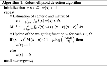
The choice of μ is paramount as it controls the number of points that are taken into account for the ellipsoid matrix estimation. It should be set to values close to  in 3D and
  in 2D (the proof is deferred in the appendix).
 in 3D and
  in 2D (the proof is deferred in the appendix).
Figure 2 shows such a process for a synthetic 2D image. The first ellipse estimate is too large as all voxels are considered but far points are progressively eliminated via the weighting function w until the algorithm converges towards the good solution. We also present results on real CEUS data in Fig. 3. The estimated ellipsoids are not perfectly accurate but robust and close enough to be used as an initialization for a segmentation algorithm.
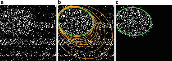


Fig. 2
(a) Original 2D synthetic image, corrupted by salt-and-pepper noise. (b) Evolution of the ellipse along the iterations (orange) and final result (green). (c) Ellipse contour and center superimposed on the product w I at convergence

Fig. 3
Results of the ellipsoid detection (red) compared to the ground truth (green), on slices of the volumes shown in Fig. 1
Kidney Segmentation via Implicit Template Deformation
The previously detected ellipsoid will now be deformed to segment the kidney more precisely. We follow the template deformation framework described in [13, 14] and extended in [15], as it is a very efficient model-based algorithm and it has already been applied successfully to kidney segmentation in CT images [16].
Implicit Template Deformation Framework
Implicit template deformation is a framework where an implicit shape defined by a function  , called the template, is deformed so that its zero level set segments a given image
  . The segmenting implicit shape is the zero level set of a function
  , therefore defined with respect to this template and a transformation of the space ψ :Ω →Ω that becomes the unknown of the problem : ϕ = ϕ0 ∘ ψ. In our application, the template is the implicit function of the previously estimated ellipsoid ϕ0 = ϕ c ∗,M ∗ and ψ is sought such that the image gradient flux across the surface of the deformed ellipsoid (ϕ0 ∘ ψ)−1(0) is maximum. The segmentation energy is then
 denotes the vector normal to the surface of the segmentation at point x.
  is a regularization term which prevents large deviations from the original ellipsoid. Its choice will be detailed in section “Transformation Model” hereafter. λ is a positive scalar parameter that controls the strength of this shape constraint.

 , called the template, is deformed so that its zero level set segments a given image
  . The segmenting implicit shape is the zero level set of a function
  , therefore defined with respect to this template and a transformation of the space ψ :Ω →Ω that becomes the unknown of the problem : ϕ = ϕ0 ∘ ψ. In our application, the template is the implicit function of the previously estimated ellipsoid ϕ0 = ϕ c ∗,M ∗ and ψ is sought such that the image gradient flux across the surface of the deformed ellipsoid (ϕ0 ∘ ψ)−1(0) is maximum. The segmentation energy is then
 denotes the vector normal to the surface of the segmentation at point x.
  is a regularization term which prevents large deviations from the original ellipsoid. Its choice will be detailed in section “Transformation Model” hereafter. λ is a positive scalar parameter that controls the strength of this shape constraint.
Using the divergence theorem, the first data-fidelity term can be rewritten as


(6)
Transformation Model
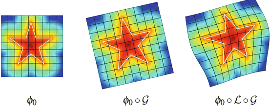
The choice of the space of possible solutions ψ to Problem (6) is, in our case, intrinsically linked to the notion of shape. A shape can be considered as a set of objects sharing the same visual aspect. It should be invariant to geometric transforms such as translation, rotation, scaling, or shearing. We will refer to such a global transformation as the pose. To set up a clear distinction between the pose and the subsequent shape deformation, similarly to [17], we design our template transformation model ψ as a functional composition of a global transformation  and a nonrigid local transformation
  (see Fig. 4):

 and a nonrigid local transformation
  (see Fig. 4):
(7)

Fig. 4
Decomposition of the transformation ψ. The implicit template ϕ0 undergoes a global transformation  and a local deformation
 and a local deformation
Pose.  is chosen as a parametric transform that coarsely aligns the template with the target surface in the image. It will basically correct or adjust the global position and scaling of the ellipsoid and can be chosen as a similarity.
  is thus represented by a matrix in homogeneous coordinates defined by 7 parameters
  and noted
  .
.
 is chosen as a parametric transform that coarsely aligns the template with the target surface in the image. It will basically correct or adjust the global position and scaling of the ellipsoid and can be chosen as a similarity.
  is thus represented by a matrix in homogeneous coordinates defined by 7 parameters
  and noted
  .
.Deformation.  is expressed using a displacement field u in the template referential
  . Similarly to problems in image registration and optical flow algorithms [18], u should be smoothly varying in space. While adding penalizations on differential terms of u to
  is a valid approach, efficient implementations are difficult to derive. Taking advantage of efficient linear filtering, smoothness of the displacement u is set as a built-in property defining it as a filtered version of an integrable unknown displacement field v
 =\int _{\varOmega }K_{\sigma }({\bf x} -{\bf y})\ {\bf v}({\bf y})\ d{\bf y} }$$](/wp-content/uploads/2016/03/A303895_1_En_2_Chapter_Equ8.gif)
where K σ is a Gaussian kernel of scale σ. The overall transformation that can therefore be parametrized by p and v will be noted ψ p,v .
 is expressed using a displacement field u in the template referential
  . Similarly to problems in image registration and optical flow algorithms [18], u should be smoothly varying in space. While adding penalizations on differential terms of u to
  is a valid approach, efficient implementations are difficult to derive. Taking advantage of efficient linear filtering, smoothness of the displacement u is set as a built-in property defining it as a filtered version of an integrable unknown displacement field v
 =\int _{\varOmega }K_{\sigma }({\bf x} -{\bf y})\ {\bf v}({\bf y})\ d{\bf y} }$$](/wp-content/uploads/2016/03/A303895_1_En_2_Chapter_Equ8.gif)
(8)
The proposed decomposition allows to define the shape prior term independently from the pose:  .
.  thus quantifies how much the segmenting implicit function ϕ deviates from the prior shape ϕ0. Using the L 2 norm we choose to constraint
  towards the identity :

The optimization problem to solve finally reads:

 .
.  thus quantifies how much the segmenting implicit function ϕ deviates from the prior shape ϕ0. Using the L 2 norm we choose to constraint
  towards the identity :
(9)

(10)
Numerical Implementation
Problem (10) is minimized via a standard gradient descent simultaneously on the parameters of the pose  and the deformation field v. The descent evolution equations are obtained by applying calculus of variations to
  . We omit the tedious details but the final equations, after a variable substitution, read
![$$\begin{cases}
\frac{\partial {\bf p}} {\partial t} = -\int _{\varOmega }\delta (\phi _{0} \circ {\mathcal L})\ .\ \left \langle \nabla \phi _{0} \circ {\mathcal L},\ (Id + J_{{\bf u}})\frac{\partial {\mathcal G}} {\partial {\bf p}}{{\mathcal G}}^{-1}\right \rangle \ .\ \varDelta I \circ {{\mathcal G}}^{-1} \\
\frac{\partial {\bf v}} {\partial t} = -\Bigg[\ \ \delta (\phi _{0} \circ {\mathcal L})\ .\ \nabla \phi _{0} \circ {\mathcal L}\ .\ \varDelta I \circ {{\mathcal G}}^{-1}\ \ + \lambda {\bf v}\Bigg] {\ast} K_{ \sigma }\\
\end{cases}$$](/wp-content/uploads/2016/03/A303895_1_En_2_Chapter_Equ11.gif)
where δ denotes the Dirac distribution and J u is the Jacobian matrix of the displacement field u.
 and the deformation field v. The descent evolution equations are obtained by applying calculus of variations to
  . We omit the tedious details but the final equations, after a variable substitution, read
![$$\begin{cases}
\frac{\partial {\bf p}} {\partial t} = -\int _{\varOmega }\delta (\phi _{0} \circ {\mathcal L})\ .\ \left \langle \nabla \phi _{0} \circ {\mathcal L},\ (Id + J_{{\bf u}})\frac{\partial {\mathcal G}} {\partial {\bf p}}{{\mathcal G}}^{-1}\right \rangle \ .\ \varDelta I \circ {{\mathcal G}}^{-1} \\
\frac{\partial {\bf v}} {\partial t} = -\Bigg[\ \ \delta (\phi _{0} \circ {\mathcal L})\ .\ \nabla \phi _{0} \circ {\mathcal L}\ .\ \varDelta I \circ {{\mathcal G}}^{-1}\ \ + \lambda {\bf v}\Bigg] {\ast} K_{ \sigma }\\
\end{cases}$$](/wp-content/uploads/2016/03/A303895_1_En_2_Chapter_Equ11.gif)
(11)
A quick analysis of Eq. (11) reveals several key aspects for an efficient implementation. Interpolating  and
and  over the whole domain Ω would be extremely time-consuming. Nevertheless, since it is multiplied by
  , the warped gradient field
  is only needed on the set
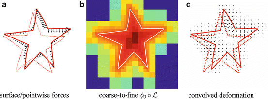
  (Fig. 5a) which highly reduces the computational burden. Moreover, precise knowledge of the warped template
  is only necessary near its zero level set. We use a coarse-to-fine approach using octrees. At each level a decision is made to further refine the cell depending on the distance measure (Fig. 5b) drastically dropping complexity. Finally, stemming from the displacement model, extrapolating image and pointwise forces to the whole space boils down to a convolution with K σ (Fig. 5c). In practice, our current 3D implementation supports up to 100 time steps per second for a discretization of the implicit function on a 64 × 64 × 64 lattice.
 and
and  over the whole domain Ω would be extremely time-consuming. Nevertheless, since it is multiplied by
  , the warped gradient field
  is only needed on the set
  (Fig. 5a) which highly reduces the computational burden. Moreover, precise knowledge of the warped template
  is only necessary near its zero level set. We use a coarse-to-fine approach using octrees. At each level a decision is made to further refine the cell depending on the distance measure (Fig. 5b) drastically dropping complexity. Finally, stemming from the displacement model, extrapolating image and pointwise forces to the whole space boils down to a convolution with K σ (Fig. 5c). In practice, our current 3D implementation supports up to 100 time steps per second for a discretization of the implicit function on a 64 × 64 × 64 lattice.
Fig. 5
Fast template deformation with coarse-to-fine distance warp and convolutions. (a) Surface/pointwise forces. (b) Coarse-to-fine  . (c) Convolved deformation
 . (c) Convolved deformation
Results for Automatic Segmentation in CEUS Images
This validation has been performed on the CEUS images of the dataset presented in section “Material”. The completely automatic pipeline had a computational time of around 5 s.
Quantitative results are reported in Fig. 6. The overall median Dice coefficient is 0.69 for the detection and 0.76 for the segmentation and 25 % of the database have a very satisfying segmentation (Dice coefficient higher than 0.85), given the very poor image quality and the presence of pathologies.
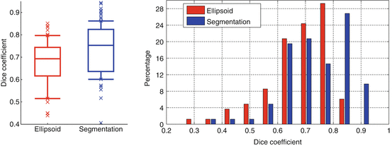

Fig. 6
Kidney detection (red) and segmentation (blue) results in terms of Dice coefficients shown as boxplots (left) and histograms (right). Boxplots show, respectively, the first decile, the first quartile, the median, the third quartile, and the ninth decile. Extreme points are shown separately
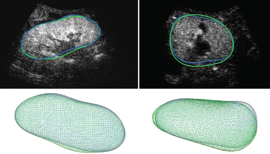
Figure 7 shows the obtained result for the two cases introduced in Fig. 1. The segmentations are very similar to the ground truth and can be considered as satisfying. Some cases are, however, more difficult (e.g., Fig. 10 in the next section) and will require additional information.
Get Clinical Tree app for offline access

Fig. 7
Result of the automatic segmentation (blue) compared to the ground truth (green) on a particular slice (top


Stay updated, free articles. Join our Telegram channel

Full access? Get Clinical Tree


