Fig. 14.1
Pulse sequence timing diagram of basic diffusion-weighted sequence formed by adding a pair of motion-probing gradients (MPGs) to a spin-echo sequence. G, Δ and δ (strength of the MPGs, time interval between the MPGs and duration of the MPGs) are adjustable parameters which influence the diffusion weighting
DW-MRI acquisition speed can be improved by using single-shot echo-planar imaging (EPI) where the whole k-space making up an image is filled within one repetition time (TR). Acquisition speed is further improved by parallel imaging methods such as SENSE and GRAPPA [20], which reduces the echo-train length. As EPI is sensitive to susceptibility artefacts [21], non-EPI techniques such as single-shot turbo spin-echo have also been used [22]. However, these are typically associated with longer acquisition times, making them less practical in a clinical setting.
14.2 b-Values and Apparent Diffusion Coefficient (ADC)
The rate of diffusion of any molecule depends on the particle size, the medium viscosity and the temperature, which can be described using the diffusion coefficient, D, with the unit mm2/s.
In a DW-MRI study, the amount of signal attenuation from each voxel after application of the MPGs is related to the strength of the MPGs and D,
![$$ \frac{S}{S_0}= \exp \left[-{\gamma}^2{G}^2{\delta}^2\left(\varDelta -\frac{\delta }{3}\right)D\right] $$](/wp-content/uploads/2016/04/A272994_1_En_14_Chapter_Equ1.gif)
where S 0 is the baseline signal with no diffusion weighting; S the signal after applying diffusion weighting; γ, G, Δ and δ the gyromagnetic ratio, strength of the diffusion gradients, time interval between the diffusion gradients and duration of the gradient, respectively; and D the diffusion coefficient. The parameters G, Δ or δ can be varied, although on clinical scanners only the gradient amplitude, G, is usually changed. In the above equation, the term  can be summarised as the b-value, b, with unit s/mm2 [23]. Thus,
(14.1)
can be summarised as the b-value, b, with unit s/mm2 [23]. Thus,(14.2)
By performing imaging using at least two b-values, it is possible to quantify the diffusion coefficient, D, for each imaged voxel
![$$ D=\frac{1}{\left({b}_2-{b}_1\right)} \ln \left[\frac{S(b{}_1{})}{S\left({b}_2\right)}\right] $$](/wp-content/uploads/2016/04/A272994_1_En_14_Chapter_Equ3.gif)
(14.3)
In tissues, in vivo water movement is influenced by various factors such as pressure gradient, ionic and osmotic gradients, capillary perfusion and bulk tissue movements. Furthermore, the motion of water is impeded by microstructures such as cell membranes and macromolecules. Thus, the measurement of diffusion coefficient, D, in tissues is only an estimation of pure water diffusivity and is termed apparent diffusion coefficient (ADC).
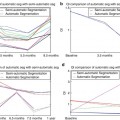
Figure 14.2 illustrates what one might expect to see in a DW-MRI study. With increasing diffusion weighting, there is progressive signal loss from the imaged voxels. ADC represents the rate of signal loss with increasing b-values; therefore if the signal intensity (in logarithmic scale) is plotted against the b-value, the slope of the resulting line represents the ADC. The steeper the slope, the higher the ADC value. The ADC value of each voxel can be displayed as greyscale or pseudo- colour on the image matrix as an ADC map.
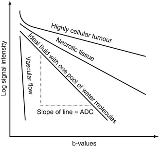
Fig. 14.2
Schematic diagram of signal attenuation of different tissue types with increasing diffusion weighting. The rate of signal loss (i.e. the slope of a line on this plot) is the ADC. Note the initial steep part of the curve seen in solid tissue (e.g. tumour), indicating the presence of a fast-moving pool of water. In tissue, this is due to pseudodiffusion, i.e. perfusion and inherent water diffusion associated with microcapillaries. If there is only one pool of water molecules, the resulting plot should be a straight line
In voxels where there is one pool of randomly moving water molecules, the rate of signal attenuation is mono-exponential and the logarithmic plot of signal intensity against b-values is a straight line (Fig. 14.2). Fitting a line onto the data points on this plot using Eq. (14.3) would yield an ADC value that is a very close approximation to the true value. Such an approach is known as a mono-exponential fit as the equation contains a single exponential. However, as demonstrated in early clinical experiments, the ADC curves tend to have an initial rapid attenuation at the low b-value ranges (b = 0–100 s/mm2) and a slower rate of attenuation at the higher b-value ranges. This has led Le Bihan et al. [23] to conclude that there exists two or more pools of randomly moving water molecules moving at different rates within tissues. Under such circumstances, ADCs derived from a mono-exponential fit would not adequately account for tissue behaviour. As such, various approaches have been developed to account for the non-mono-exponential attenuation of signal in tissues.
14.3 Pseudodiffusion and Intravoxel Incoherent Motion (IVIM)
As well as diffusion of water molecules within tissues, bulk water movement in randomly orientated capillaries (i.e. perfusion) can also cause phase dispersion at DW-MRI. The resulting loss of signal is akin to that seen in true diffusion and has been termed pseudodiffusion [23]. As capillary flow is significantly faster compared with water diffusion in tissue, signal loss per unit increase in b-value is also greater, meaning that signal loss from the majority of perfusing water molecules occurs at relatively low b-values (b = 0–100 s/mm2). If the low b-values are included in a mono-exponential calculation of ADC, the value of ADC would be overestimated, i.e. the ADC would suggest a higher diffusion rate than can be accounted for by tissue water. Since the effect of perfusion on ADC is particularly marked at low b-value ranges, a means to desensitise the effect of perfusion has been suggested by calculating ADC from the higher b-value ranges (b > 100 s/mm2), to produce a perfusion insensitive ADC. In contrast, an ADC value calculated using a full range of b-values is variably perfusion sensitive ADC [24–26] (Fig. 14.3), depending on the number and range of b-values used for its calculation.
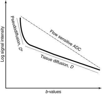
Fig. 14.3
Schematic DW-MRI signal plot of a generic soft tissue demonstrating perfusion and diffusion effects. If the rate of signal loss (ADC) is calculated from all b-values, the resulting ADC is sensitive to flow and overestimates the true diffusivity. In tissues with significant perfusion fraction, tissue diffusion can be more accurately approximated using the bi-exponential model or by omitting the low b-values in the ADC calculation
A more sophisticated approach accounting for pseudodiffusion has been proposed by Le Bihan et al. [23, 27, 28]. In this approach, water molecules in random motion are said to exhibit intravoxel incoherent motion (IVIM), which include water molecules undergoing true diffusion and those moving within randomly orientated capillaries (perfusion). The contribution of true diffusion and perfusion towards signal loss are written as two separate terms in the equation modified from (14.2),
where f V is the fractional volume of flowing water molecules within the capillaries (therefore, (1 − f V) denotes the fraction of water molecules undergoing true diffusion); D is the tissue diffusion coefficient, uninfluenced by movement of water molecules within the capillaries; D* is the pseudodiffusion coefficient that represents the amount of non-diffusional random movements of water molecules, e.g. perfusion, plus the diffusion of these water molecules. As discussed in the above section, there is minimal contribution from pseudodiffusion at the higher b-values, thus the term  becomes negligible at the higher b-value ranges. By performing the DW-MRI study with a range of b-values, including b = 0 s/mm2, a number of b-values between 0 and 100 s/mm2 and higher b-values, it is possible to solve the bi-exponential equation (14.4) for D, D* and f V. ADC can be approximated as
(14.4)
becomes negligible at the higher b-value ranges. By performing the DW-MRI study with a range of b-values, including b = 0 s/mm2, a number of b-values between 0 and 100 s/mm2 and higher b-values, it is possible to solve the bi-exponential equation (14.4) for D, D* and f V. ADC can be approximated as(14.5)
Using the IVIM model, it is therefore possible to attribute a fast component of tissue water diffusivity to perfusion by deriving D* and f V (Fig. 14.3). Indeed, studies comparing intravascular tracer and DW-MRI with IVIM modelling have shown good correlation between tissue blood volume and f V and between relative blood flow and D* [29, 30]. Of note is that a tissue may have high D* but low f V values, as the two vascular properties are not related. However, as the pseudodiffusion coefficient, D*, is influenced by physiological processes other than perfusion, e.g. glandular secretion and renal tubular flow, there remains controversy regarding the reliability of IVIM-derived perfusion parameters in secretory organs such as the salivary glands and kidneys [31–33].
14.4 Other Non-mono-exponential Diffusion Models
Another approach to account for the non-mono-exponential attenuation of the water signal in tissue is the stretched-exponential model [34], which does not necessitate a priori knowledge of the number of diffusion pools. The amount of signal loss after application of MPGs is described as thus
where DDC is the distributed diffusion coefficient, a surrogate for ADC, and α is the stretching parameter which describes the deviation of the curve from a mono-exponential line. α = 1 describes perfect alignment with the mono-exponential line consistent with a single diffusion pool, whereas a value of α < 1 suggests the presence of a distribution of different diffusion rates within the imaged voxel. Hence, α is also known as a heterogeneity index. One limitation of the stretched-exponential model is that unlike the IVIM model, it is difficult to correlate the term of α with a specific biological underpinning.
(14.6)
There are other phenomenological diffusion models (e.g. Gaussian, Kurtosis) that are used in research, but these are beyond the scope of discussion in this chapter.
14.5 Technical Implementation
14.5.1 General Considerations
DW-MRI is made possible within a clinically acceptable time frame with EPI and parallel imaging. However, T2* effects of the tissues causes signal attenuation on EPI and is sensitive to B0, leading to reduced signal-to-noise ratio (SNR). This can be improved by increasing the slice thickness, increasing the number of signal averages, increased pixel size or large field of view (FOV), shorter echo-times, optimising receiver bandwidth and use of parallel imaging techniques.
Another problem in DW-MRI is chemical shift artefacts from fat which can be particularly pronounced on DW-MRI images due to the narrow bandwidth used in phase encoding. As the bandwidth per pixel in DW-MRI is 10–30 Hz compared to the fat-water chemical shift frequency of 220 Hz, signal displacement up to 10–15 pixels can be seen (approximately 6 cm if a pixel size of 4 mm is used). Ensuring optimal fat signal suppression is therefore critical in DW-MRI.
With increasing availability of 3.0 T scanners, there is a potential to improve image quality with the theoretical doubling of SNR compared to a 1.5 T system. However, at higher field strength, susceptibility artefacts are accentuated and become more problematic. Chemical shift artefacts can also be more profound.
14.5.2 DW-MRI in the Body
Breathing-related artefacts are an additional consideration in body DW-MRI. This problem can be dealt with in three approaches [35]: (1) breath-hold imaging, (2) navigator echo respiratory-triggered imaging and (3) free breathing.
Breath-hold DW-MRI acquisition time is typically <20 s per breath hold and the full dataset is acquired in a few breath holds. It may improve conspicuity of small lesions but has the disadvantage of limited b-values per breath hold, increased sensitivity to susceptibility artefacts (due to long echo train) and reduced SNR. Images are also prone to degradation by other uncontrolled physiological motions such as vessel/cardiac pulsation and peristalsis.
In navigator echo respiratory-triggered imaging [36], the position of the diaphragm is tracked by a pencil-beam excitation prepulse placed between the liver and lung. Compared with breath-hold imaging, navigator DW-MRI shows higher SNR and lesion to liver contrast ratio [37]. In a modified sequence using navigator echo to track pixel displacement without respiratory gating, image sharpness is improved compared with free-breathing technique with minimal increase in acquisition time [38, 39].
Free-breathing technique uses multiple signal averaging to overcome the effect of motion. Because of the increased number of acquisitions, it has better SNR compared with breath-hold imaging and allows more b-values to be acquired. It is also possible to use thinner slices in free breathing, thereby allowing for multiplanar manipulation of the images. ADC obtained using free-breathing technique has been found to be reproducible and not dissimilar to values obtained using other acquisition techniques [40, 41]. Typical image acquisition protocols used for body DW-MRI are shown in Table 14.1.
Table 14.1
Single-shot DW-EPI parameters in clinical examination of the abdomen and pelvis
Abdomen | LFOV pelvis | SFOV pelvis | |
|---|---|---|---|
Field of view (mm) | 380 | 380 | 220–280 |
RFOV | 80 | 80 | 80 |
Number of slices | 26–33 | 40–48 | 18 |
Slice thickness (mm) | 6–7 | 6 | 5 |
Slice gap (mm) | 10 % | 10 % | 10 % |
Matrix | 104–112/256 | 104–112/256 | 112/256 |
Foldover direction | AP | AP | AP |
TE (ms) | 66–70 | 66 | 66–70 |
TR (ms) | 5,000 | 5,600–7,400 | 2,500–3,100 |
PI factor | 2 | 2 | 2 |
Fat saturation | SPAIR | IR/SPAIR | SPAIR |
EPI factor | 59–104 | 59–104 | 75–112 |
Signal averages | 4–5 | 4 | 4–8 |
Bandwidth (Hz/Px) | 1,800 | 1,800 | 1,800 |
b-values (s/mm2) | 0,100,500,750 | 0,900 | 0,300,750 |
Acquisition time (min) | 4.5 | 2.5 | 3 |
14.6 Image Interpretation
Interpretation of DW-MRI and its accompanying ADC maps can be performed qualitatively by visual assessment or quantitatively by numerical analysis of regions of interest (ROIs) on the ADC maps. When visually assessing the DW-MRI images, the images should be interpreted together with the ADC map and other morphological MR images to avoid misinterpretation. Likewise, when quantitatively analysing the ADC map, the source diffusion-weighted images and other morphological images should be assessed for any artefacts, which may bias the ADC estimates.
Most DW-MRI studies will yield observations that fit into one of the following four categories (Fig. 14.4) as below.
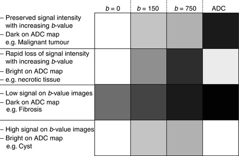
Fig. 14.4
Four common signal intensity patterns observed on the b-value images and ADC maps at DWI
1.
Lesions with relatively preserved signal intensity with increasing b–values and dark on ADC maps (Fig. 14.5). This indicates impeded diffusion within the lesion and may result from increase in cellular density and/or increased tortuosity of the extracellular space. Malignancy is the prime example of pathology, which may give rise to this picture. Other pathologies that may lead to this imaging appearance include active inflammation [42] and abscess [43].
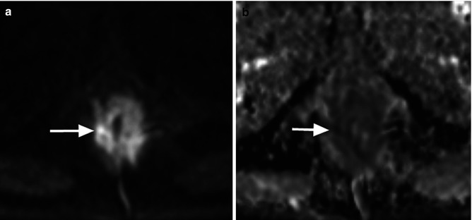
Fig. 14.5
A man with carcinoma of the anus. (a) b = 900 s/mm2 DWI image shows abnormal high signal and thickening of the anal canal (arrow). (b) ADC map returns low signal intensity and ADC values (arrow)
2.
Lesions showing rapidly decreasing signal intensity with increasing b–values and bright on ADC maps (Fig. 14.6). This occurs in lesions with relatively unimpeded diffusion, e.g. cysts, necrotic tissues and vasogenic oedema without accompanying rise of cellularity. Careful interpretation of the DW-MRI and morphological images may reveal clues as to the true nature of the lesion. In simple cysts, it would be unusual to observe perilesional diffusion impediment or complex internal structure; conversely, one might expect to see a rim of tissue with impeded diffusion in necrotic tumour, which represents viable disease.
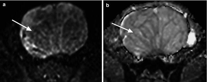
Fig. 14.6
A woman with cystadenoma of the ovary. (a) The cystic area within the lesion shows signal loss on the b = 750 s/mm2 image (arrow) compared with the internal septi which remains relatively high signal. (b) The cystic area returns high ADC values on the ADC map (arrow)
3.
Lesions showing low signal intensity on both the b–value images and ADC map (Fig. 14.7). This can be observed in regions of inherent low signal on the fat-suppressed T2-weighted image (e.g. fat and fibrosis) or may be secondary to imaging artefacts (including processes that result in susceptibility effects in the local magnetic field such as haemorrhage, iron deposition and dense calcifications). Note, however, that fibrosis can exhibit a range of signal intensities and ADC values and is yet to be fully characterised.
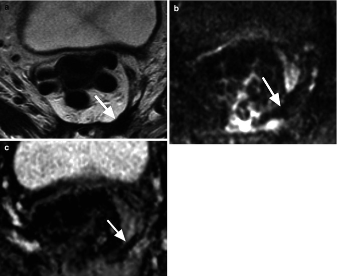
Fig. 14.7
A man with previous low anterior resection for rectal cancer. (a) T2-weighted MRI shows low signal intensity change in the presacral area (arrow) consistent with fibrosis. (b) This shows low signal intensity on the b = 900 s/mm2 image (arrow) and (c) also returns predominantly low ADC value (arrow)
4.
 New Therapies and Functional-Molecular Imaging
 Overview of Functional MR, CT, and US Imaging Techniques in Clinical Use
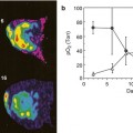 MRI Hypoxia Measurements
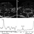
 Spectroscopy of Cancer
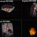
 Current Clinical Imaging of Hypoxia with PET and Future Perspectives
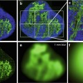
 Medical Image Computing for Oncology: Review and Clinical Examples


Lesions showing relatively preserved signal intensity with increasing b–values and bright on ADC map (Fig. 14.8). This results from “T2 shine-through” effects and will be discussed in the next section.
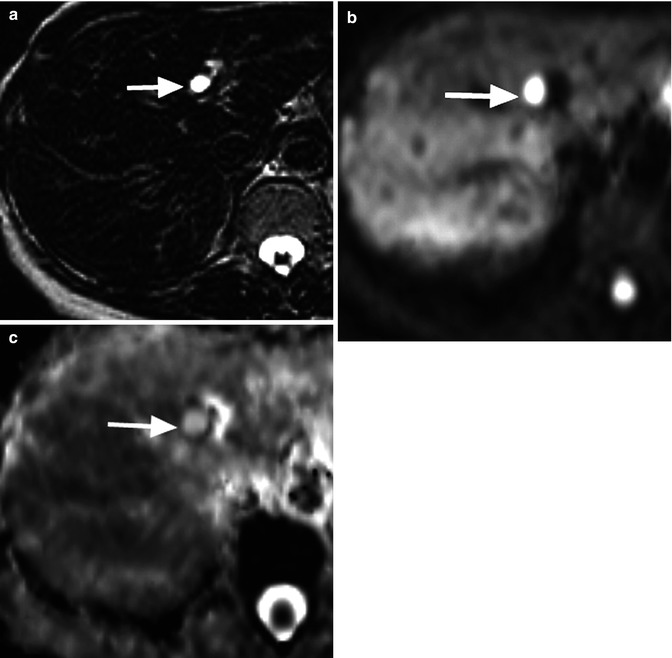
Fig. 14.8
A 40-year-old man with a cyst in the left lobe of the liver. (a) T2-weighted image obtained with long echo time (TE = 240 ms) shows a 1 cm high signal intensity cyst in left hepatic lobe (arrow). (b) The cyst remains high signal on the b = 750 s/mm2 image due to its long T2 relaxation time (arrow). (c) Note the high ADC value of cyst confirming T2 shine-through effect (arrow)
Related posts:
New Therapies and Functional-Molecular Imaging
Overview of Functional MR, CT, and US Imaging Techniques in Clinical Use
MRI Hypoxia Measurements
Spectroscopy of Cancer
Current Clinical Imaging of Hypoxia with PET and Future Perspectives
Medical Image Computing for Oncology: Review and Clinical Examples
Stay updated, free articles. Join our Telegram channel
Full access? Get Clinical Tree
