Fig. 1
The database used in this chapter has thousands of 3D CT scans with different body regions and severe pathologies
Landmark Detection Methods
State-of-the-art landmark detection methods are based on statistical learning [50]. In this paradigm, each landmark has a dedicated detector [32, 55]. In [37], volumes have consistent field of view, e.g., the database consists of only liver scans. In such a case, it is possible to predefine a region of interest (ROI) for each landmark detector. In general, however, the position of each landmark can vary significantly across different scans; in most cases, some landmarks such as the head or toe are not even present in a body scan. Under such cases, running multiple detectors independently of each other can result in false detections [32, 39]. To handle the problem of false detections, one can exploit the spatial relationship information between landmarks to reduce false detections. A model for describing the spatial relationship between landmarks is the Markov Random Field [4, 5].
Another important factor to consider when designing multiple landmark detectors is speed. Naively running each detector on the whole volume yields a time complexity proportional to the number of detectors and volume size. This poses significant computational resources when the number of landmarks of interest is large, or when the volumes are large. More efficient detection can be achieved with a sequential method [32]. This method assumes at least one of the landmark positions is known. Since the relative positions of landmarks in the human body are constrained (e.g., the kidney is below the heart in a typical CT scan), one can define a search range (sub-volume) for each unknown landmark relative to the known landmark positions. Detecting a landmark within a local search range instead of within the whole volume achieves faster speed.
In practice, however, none of the landmark positions is known a priori, and therefore the sequential method described above needs some pre-processing work to find the first landmark, also called the anchor landmark [32]. There are two major difficulties in finding the anchor landmark. First, as mentioned earlier, detectors are prone to false positives when used alone. This poses a chicken-and-egg problem: To find the anchor landmark robustly, we need to rely on the positions of other landmarks, which are, however, unknown. A second problem exists, even if the detectors had zero false positive rates: typical CT scans have small (partial) field-of-view, as opposed to imaging the whole body from head to toe. Since we do not know which landmarks are present in a partial field-of-view volume, it would require trying many detectors, each one running in the whole volume, until a landmark is found present. This process is a computational bottleneck of the sequential method. In other words, the key problem in the sequential method is to find the anchor landmark robustly and efficiently. This brings us to the topic of context exploitation in the next section.
Context Exploitation
Designing a useful landmark detection method should effectively exploit the rich contextual information manifested in the body scans, which can be generally categorized as unary (or first-order), pairwise (or higher-order), and holistic context.
The unary context refers to the local regularity surrounding a single landmark. The classical object detection approach in [49, 50] exploits the unary context to learn a series of supervised classifier to separate the positive object (herein landmark) from negative background. The complexity of this approach depends on the volume size.
The pairwise or higher-order context refers to the joint regularities between two landmarks or among multiple landmarks. Liu et al. [32] embed the pairwise spatial contexts among all landmarks into a submodular formulation that minimizes the combined search range for detecting multiple landmarks. Here the landmark detector is still learned by exploiting the unary context. In [55], the pairwise spatial context is used to compute the information gain that guides an active scheduling scheme for detecting multiple landmarks. Seifert et al. [44] encoded pairwise spatial contexts into a discriminative anatomical network.
The holistic context goes beyond the relationship among a cohort of landmarks and refers to the whole relationship between all voxels and the landmarks; in other words, regarding the image as a whole. In [58], shape regression machine is proposed to learn a boosting regression function to predict the object bounding box from the image appearance bounded in an arbitrarily located box and another regression function to predict the object shape. Pauly et al. [38] simultaneously regress out the locations and sizes of multiple organs with confidence scores using a learned Random Forest regressor. To some extent, image registration [22] can be regarded as using the holistic context.
In [32], no holistic context is used. Instead, the aforementioned “anchor landmark” is searched to trigger the whole detection process. There are two major problems of finding the anchor landmark. First, as mentioned earlier, detectors are prone to false positives when used alone. Detecting the “anchor landmark” utilizes only the unary context in exhaustive scanning. Since any false positive detection of the “anchor landmark” causes catastrophe in detecting the remaining ones, sometimes it requires trying many detectors, each one running in the whole volume, until a landmark is found present.
In this chapter we present an approach that leverages all three types of contexts. It consists of two steps:
The first step uses nearest neighbor (NN) matching, which exploits holistic context to perform matching and transfers landmark annotations. This is significantly different from the regression approach as in [58] which scans through the image searching for landmarks. This is also different from the “anchor landmark” approach in [32]. Detecting the “anchor landmark” utilizes only the unary context in exhaustive scanning. Since any false positive detection of the “anchor landmark” causes catastrophe in detecting the remaining ones, sometimes it requires trying many detectors, each one running in the whole volume, until a landmark with very high confidence score is found. Finally we achieve a much faster algorithm for detecting landmarks.
The second step uses submodular optimization to minimize overall computation time. The method exploits both unary and pairwise contexts and aims to minimize the overall computation. The approach was first introduced in [32] to minimize the total search range and later extended to minimize overall computation time in [31] by modifying the cost function in the submodular formulation.
Coarse Landmark Detection Using Nearest Neighbor Matching
Our method consists of two steps. The first step is coarse detection and involves finding a rough position estimate for all landmarks. After coarse detection, we refine the landmark positions through landmark detectors. This section focuses on the coarse detection step.
Assume that a volume is represented by a D-dimensional feature vector. Given a query (unseen input) vector x ∈ R D , the problem is to find the element y ∗ in a finite set Y of vectors to minimize the distance to the query vector:

where d(.,.) is the Euclidean distance function. Other choices can be used too. Once y ∗ is found, the coarse landmark position estimates are obtained through a “transfer” operation, to be detailed in section “Transferring Landmark Annotations”.

(1)
Volume Features
To facilitate the matching, we represent each volume by a D-dimensional feature vector. In particular, we adopt a representation of the image using “global features” that provide a holistic description as in [47], where a 2D image is divided into 4 × 4 regions, eight oriented Gabor filters are applied over four different scales, and the average filter energy in each region is used as a feature, yielding in total 512 features. For 3D volumes, we compute such features from nine 2D images, consisting of the sagittal, axial, and coronal planes that pass through 25 %, 50 %, and 75 % of the respective volume dimension, resulting a 4,608-dimensional feature vector.
Efficient Nearest Neighbor Search
In practice, finding the closest (most similar) volume through evaluating the exact distances is too expensive when the database size is large and the data dimensionality is high. Two efficient approximations are used for speedup. Vector quantization [33] is used to address the database size issue and product quantization [24] for the data dimensionality issue.
A quantizer is a function q(.) mapping a D-dimensional vector x to a vector  . The finite set Q is called the codebook, which consists of K centroids. The set of vectors mapped to the same centroid forms a Voronoi cell, defined as
  . The K Voronoi cells partition the space of R D . The quality of a quantizer is often measured by the mean squared error between an input vector and its representative centroid q(x). We use the K-means algorithm [33] to find a near-optimal codebook. During the search stage, which has high speed requirement, distance evaluation between the query and a database vector consists of computing the distance between the query vector and the nearest centroid of the database vector.
 . The finite set Q is called the codebook, which consists of K centroids. The set of vectors mapped to the same centroid forms a Voronoi cell, defined as
  . The K Voronoi cells partition the space of R D . The quality of a quantizer is often measured by the mean squared error between an input vector and its representative centroid q(x). We use the K-means algorithm [33] to find a near-optimal codebook. During the search stage, which has high speed requirement, distance evaluation between the query and a database vector consists of computing the distance between the query vector and the nearest centroid of the database vector.
These volume feature vectors are high dimensional (we use D = 4,608 dimensions), which poses difficulty for a straightforward implementation of the K-means quantization described above. A quantizer that uses only 1∕3 bits per dimension already has 21536 centroids. Such a large number of centroids make it impossible to run the K-means algorithm in practice. Product quantization [24] addresses this issue by splitting the high-dimensional feature vector into m distinct sub-vectors as follows,

The quantization is subsequently performed on the m sub-vectors q 1(u 1(x)),…,q m (u m (x)), where q i , i = 1,…,m denote m different quantizers. In the special case where m = D, product quantization is equivalent to scalar quantization, which has the lowest memory requirement but does not capture any correlation across feature dimensions. In the extreme case where m = 1, product quantization is equivalent to traditional quantization, which fully captures the correlation among different features but has the highest (and practically impossible, as explained earlier) memory requirement. We use m = 1,536 and K = 4 (2 bits per quantizer).

(2)
A Note on Product Quantization and Related Work
The explosion of the amount of digital content has stimulated search methods for large-scale databases. An exhaustive comparison of a query with all items in a database can be prohibitive. Approximate nearest neighbors (ANN) search methods are invented to handle large databases, at the same time seeking a balance between efficiency and accuracy. Such methods aim at finding the nearest neighbor with high probability. Several multi-dimensional indexing methods, such as KD-tree [16], have been proposed to reduce the search time. However, for high-dimensional feature vectors, such approaches are not more efficient than the brute-force exhaustive distance calculation, whose complexity is linear with the database size and the data representation dimension [24].
One of the most popular ANN techniques is Locality-Sensitive Hashing [10]. However, most of these approaches are memory consuming. The method of [54] embeds the vector into a binary space and improves the memory constraint. However, it is outperformed in terms of the trade-off between accuracy and memory usage by the Product Quantization method [24].
Volume Size Clustering
The anisotropic resampling of volumes into the same size, as done in section “Volume Features”, causes distortion in appearance. This could have negative impact on nearest neighbor search. For example, when a head scan and a whole body scan are resampled to the same number of voxels, their appearances could become more similar than they were in their original sizes, and hence negatively affecting the results in Eq. (1). We use the K-means algorithm [33] to cluster all database volumes into 30 categories based on the volume’s physical dimensions. Given a query volume, it is first assigned to the category of volumes with similar physical sizes. Nearest neighbor search is then only performed within this category.
Transferring Landmark Annotations
Given a query, we use the aforementioned method to find the most similar database volume. Assume this database volume consists of N landmarks with positions {s 1,…,s N }. We simply “transfer” these landmark positions to the query, as illustrated in Fig. 2. In other words, the coarsely detected landmark positions are set as {s 1,…,s N }. In the next section, we discuss how to refine these positions.
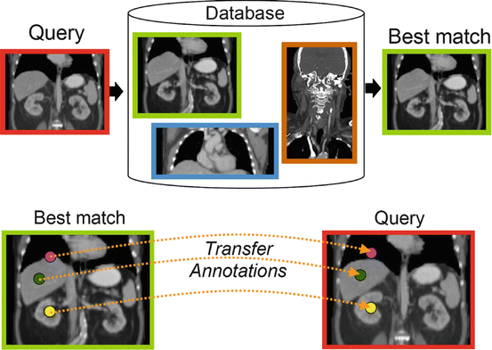

Fig. 2
Coarse landmark detection, a 2D illustration. Real system operates on 3D volumes. Upper figure: nearest neighbor search. Lower figure: annotated positions of database volume are transferred to query. The real system operates on 3D volumes
Fine Landmark Detection with Submodular Optimization
After the step of NN matching, certain landmarks are located roughly. We now trigger the landmark detectors to search for a more precise position for each landmark only within local search ranges predicted from the first stage results. Running a landmark detector locally instead of over the whole volume reduces the computation and also reduces false positive detections. The local search range of each detector is obtained off-line based on spatial statistics that capture the relative position of each pair of landmarks. Note that the two sets of landmarks in two stages can be different.
In order to speed up the detection, the order of triggering the landmark detectors needs to be considered. This is because, once a landmark position is refined by a detector, we can further reduce the local search ranges for the other landmarks by using the pairwise spatial statistics that embody the pairwise context.
The main goal in this section is to minimize the computational cost of multiple landmark detection. The computational cost is controlled by (1) the size of the image subspace (or search space) in which a detector is performing the search and (2) the unit cost of the landmark detector. We will first focus on item (1), and later extend the framework to item (2).
Having n landmarks detected, with N − n landmarks remaining to detect, which detector should one use next, and where should it be applied, so that the overall computational cost is minimized? These two questions are tightly related, and the answer is simple: determine the search space for each detector based on the already detected landmarks and pick the detector that has the smallest search space. We will show theoretical guarantees of the algorithm in section “Greedy Algorithm”, and then in section “Another Search Space Criteria” extend the algorithm to take multiple factors into account, including the size of the search space and the unit cost of the detector (classifier).
Search Space
In sequential detection, landmarks already detected provide spatial constraints on the landmarks remaining to be detected. Consider an object consisted of N distinct landmarks. Denote by

the ordered set of detected landmarks. Denote by U the un-ordered set of landmarks that remains to be detected. For each landmark l i ∈ U, its search space  is determined jointly by landmarks in Λ (1):(n), for example, by the intersection of the individual search spaces,

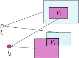
where  denotes the search space for landmark l i conditioned on the position of a detected landmark l j . This is illustrated in Fig. 3. This definition could be restrictive, so we will discuss alternatives in sections “Another Search Space Criteria” and “Multiple Search Space Criteria”.

(3)
 is determined jointly by landmarks in Λ (1):(n), for example, by the intersection of the individual search spaces,
(4)
 denotes the search space for landmark l i conditioned on the position of a detected landmark l j . This is illustrated in Fig. 3. This definition could be restrictive, so we will discuss alternatives in sections “Another Search Space Criteria” and “Multiple Search Space Criteria”.
Fig. 3
Illustration of the search space definition in Eq. (4). Detected landmarks l 1 and l 2 provide search spaces for un-detected landmarks l 3 and l 4 (not shown). Final search spaces V 3 and V 4 for l 3 and l 4 are obtained by intersection. A greedy algorithm would prefer landmark l 4 over l 3 as the next landmark to detect since V 4 is smaller than V 3
Denote the search volume (or search area) of search space  as
as  , which calculates the volume of
  . Without loss of generality, assume the search volume is the cardinality of the set of voxels (pixels) that fall within the search space. Define the constant Ω ϕ ≡ Ω k (ϕ),∀k, as the space of the whole image, which is a tight upper bound of the search space. The search volume has the following property:
 as
as  , which calculates the volume of
  . Without loss of generality, assume the search volume is the cardinality of the set of voxels (pixels) that fall within the search space. Define the constant Ω ϕ ≡ Ω k (ϕ),∀k, as the space of the whole image, which is a tight upper bound of the search space. The search volume has the following property:
Theorem 1
∀S ⊆ T,


(5)
Set functions satisfying the above property are called supermodular [43].
Let us simplify the notation by omitting the subscript l i from  . Define the complement
  , where Ω ϕ has earlier been defined as the space of the whole volume.
 . Define the complement
  , where Ω ϕ has earlier been defined as the space of the whole volume.
Lemma 1
Ω(S ∪{ l}) = Ω(S) ∩ Ω({l})
This follows from the definition.
Lemma 2
If S ⊆ T, then Ω(S) ⊇ Ω(T)
Proof T = S ∪ (T ∖ S) ⇒ From Lemma 1,  .
.
 .
.Lemma 3

Proof  = RHS.
 = RHS.
Lemma 4
If Ω(T) ⊆ Ω(S), then 

Lemma 5
If Ω(T) ⊆ Ω(S), then V (Ω(T) ≤ V (Ω(S))
Finally we prove the supermodularity of V (Ω(.)) in Theorem 1.
Proof of Theorem 1 From Lemma 2, Ω(S) ⊇ Ω(T). Then  . From Lemma 3, we have Ω(S) ∖ Ω(S ∪{ l}) ⊇ Ω(T) ∖ Ω(T ∪{ l}). From Lemma 5, we have V (Ω(S) ∖ Ω(S ∪{ l})) ≥ V (Ω(T) ∖ Ω(T ∪{ l})). From Lemma 4, Q.E.D.
 . From Lemma 3, we have Ω(S) ∖ Ω(S ∪{ l}) ⊇ Ω(T) ∖ Ω(T ∪{ l}). From Lemma 5, we have V (Ω(S) ∖ Ω(S ∪{ l})) ≥ V (Ω(T) ∖ Ω(T ∪{ l})). From Lemma 4, Q.E.D.
Proof From Lemma 2 and Lemma 5, we have ∀S ⊆ T, we have V (Ω(T)) ≤ V (Ω(S)), which shows V (.) is nonincreasing. Consequently, F(.) is nondecreasing.
Greedy Algorithm
The goal is to find the ordered set Λ (2):(N) that minimizes the cumulated search volume, i.e. ,

Note that in Eq. (11) we do not include the first landmark l 1 as its search space is typically the whole image when no landmarks have been detected a priori. The first landmark can be detected using the method in section “Transferring Landmark Annotations”, or by the method in section “Finding the Anchor Landmark”. We will discuss these different methods in detail in section “Comparing Holistic-Anchoring and Sequential-Anchoring”.

(6)
Define the cost function C k (Λ) = V (Ω k (Λ)),∀k. A greedy algorithm for finding the ordering {l (1),…,l (N)} that attempts to minimize the overall cost is to iteratively select the detector that yields the smallest cost. This is illustrated in Fig. 4 and proceeds as follows.
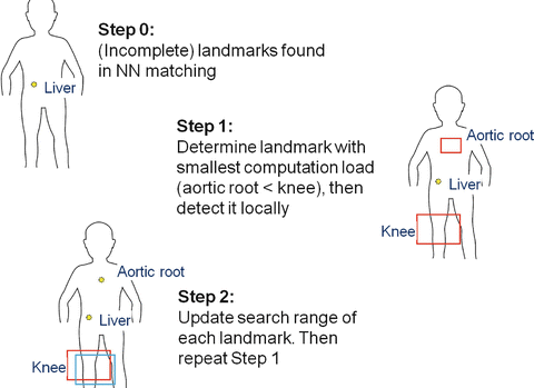

Fig. 4
Illustration of the greedy algorithm. Different box colors (red and blue) indicate search ranges provided by other landmarks (liver and aortic root)

This simple algorithm has nice theoretical properties. Define

Hence, F k (ϕ) = 0. From Lemma 6, F k (.) is a nondecreasing set function. From Eq. (1) and (7), ∀S ⊆ T,

which means F k (.) is submodular [43]. Furthermore, since C k (ϕ) is constant over k, Eq. (11) becomes


(7)

(8)

(9)
Together, these properties bring us to the theorem that states the theoretical guarantee of the greedy algorithm.
Theorem 2
If F(.) is a submodular, nondecreasing set function, and F(ϕ) = 0, then the greedy algorithm finds a set Λ′, such that  [36].
[36].
 [36].
[36].Optimizing submodular functions is in general NP-hard [34]. One must in principle calculate the values of N! detector ordering patterns. Yet, the greedy algorithm is guaranteed to find an ordered set Λ such that F(.) reaches at least 63 % of the optimal value.
Note that the ordering found by the algorithm is image-dependent, since the search space of the next detector is dependent on the position of the landmarks already detected. Therefore, the algorithm is not performing an “off-line” scheduling of detectors. For another example, when the search space of a landmark is outside the image or if its detection score is too low, then this landmark is claimed missing. This would influence the subsequent detectors through the definition of the search space and affect the final ordering.
Another Search Space Criteria
Another useful definition of search space can be defined as follows:

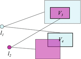
In each round of the greedy algorithm, each detected landmark provides a search space candidate for each un-detected landmark. Each un-detected landmark then selects the smallest one among the provided candidates. The greedy algorithm then selects the un-detected landmark that has the smallest search space. This is illustrated in Fig. 5. We call this search space criteria the min-rule, and the one in section “Search Space” the intersection-rule.

(10)

Fig. 5
Illustration of the search space definition in Eq. (10). Detected landmarks l 1 and l 2 provide search spaces for un-detected landmarks l 3 and l 4 (not shown). Final search spaces V 3 and V 4 for l 3 and l 4 are the minimum sets. This time, a greedy algorithm would prefer landmark l 3 over l 4 as the next landmark to detect since V 3 is smaller than V 4
Denote  as the landmark in the set of detected landmarks S that provides the smallest search range for detector l i . Here we show that this definition also satisfies Theorem 1.
 as the landmark in the set of detected landmarks S that provides the smallest search range for detector l i . Here we show that this definition also satisfies Theorem 1.
Lemma 8
∀S ⊆ T,V (Ω(S)) ≥ V (Ω(T))
Proof From definition, Ω(S) = min l∈S Ω({l}), and Ω(T) = min l∈T Ω({l}). Since S ⊆ T, we have Ω(S) ≥ Ω(T), and hence V (Ω(S)) ≥ V (Ω(T)).
Proof of Theorem 1
Case (i):
 . This means including l does not decrease the search space, and hence V (Ω(T)) = V (Ω(T ∪{ l})). But from Lemma 8, V (Ω(S)) ≥ V (Ω(S ∪{ l})) always holds. Hence
  .
.
 . This means including l does not decrease the search space, and hence V (Ω(T)) = V (Ω(T ∪{ l})). But from Lemma 8, V (Ω(S)) ≥ V (Ω(S ∪{ l})) always holds. Hence
  .
.Case (ii):
 . This means l provides a smaller search space than any other landmark in T, and hence
  . Since S ⊆ T, we also have
  . Hence, V (Ω(S ∪{ l})) = V (Ω(T ∪{ l})). But from Lemma 8, V (Ω(S)) ≥ V (Ω(T)) always holds. Hence
  .
.
 . This means l provides a smaller search space than any other landmark in T, and hence
  . Since S ⊆ T, we also have
  . Hence, V (Ω(S ∪{ l})) = V (Ω(T ∪{ l})). But from Lemma 8, V (Ω(S)) ≥ V (Ω(T)) always holds. Hence
  .
.Multiple Search Space Criteria
Since submodularity is closed under linear combination with nonnegative scalars [43], multiple submodular functions can be optimized simultaneously. For example, one could combine the min-rule and intersection-rule. Note that the set of individual search spaces  need not be the same for the min- and intersection-rules. Under this combination, some detectors could obtain a search range from the min-rule, and some from the intersection-rule.1 , 2
 need not be the same for the min- and intersection-rules. Under this combination, some detectors could obtain a search range from the min-rule, and some from the intersection-rule.1 , 2
 Cost of Detector
The algorithm introduced so far only considered the search space. In practice, different detectors have different costs and this should be taken into account during optimization. For example, if we have two detectors, then the algorithm above would select the next detector that has a smaller search space. However, this detector might have a much higher unit computational cost due to, for example, higher model complexity. One should multiply (and not linearly combine) search volume with the unit cost, since a detector is applied to each voxel within the search space and only the product reflects the cost correctly.
Fortunately, multiplication of a submodular function by a nonnegative scalar also maintains submodularity [43]. Denote q i as the computational cost of detector i. The product  then considers the joint computational cost. Since
  is submodular, the greedy algorithm can be applied and the same theoretical guarantees still hold.
 then considers the joint computational cost. Since
  is submodular, the greedy algorithm can be applied and the same theoretical guarantees still hold.
The computational cost of a detector (classifier) can be estimated from, for example, the number of weak learners in boosting-based classifiers [50], the expected number of classifiers in a cascade of classifiers [50], or the empirical running time. Denote by α[l j ] the unit computation cost for evaluating the detector for landmark l j . The goal is then to find the ordered set Λ (1):(N) that minimizes the total computation


Stay updated, free articles. Join our Telegram channel

Full access? Get Clinical Tree


