Fig. 1
Framework of registration evaluation
In the procedure of landmark detection, firstly, 3D SIFT keypoint detection [14, 20], which detects local extrema from image pyramids consisting of differences in Gaussian-blurred images at multiple scales, is applied to the fixed image.
After the SIFT feature points detection in the fixed image, a 3D phase-based image matching algorithm is developed to match the corresponding landmarks in the registered moving image. A discrete Fourier transform (DFT) of image blocks around SIFT feature points and that of their candidate correspondences is computed, respectively. Phase components of the image-block pairs in the frequency domain are used to estimate locations of the correspondences. The image-block matching method can achieve high accuracy at the sub-voxel level [15, 29]. Even under rotation, the matching method can give good performance by coarse-to-fine and iterative procedures. As a result, it is possible to measure a registration error by using the distance between the SIFT keypoints and their correspondences. Note that although this work focuses on registration validation on thoracic CT images, the proposed method can be extended to different types and modalities of images, since both the feature detection and image matching algorithms can be applied to general image data.
Feature Point Detection
In this work, a 3D landmark detector is required to extract fiducial landmarks as reference points for spatial accuracy evaluation of image registration. Harkens et al. [16] investigated nine 3D differential operators for the detection of anatomical landmarks in medical images. Recently, the SIFT detector and descriptor introduced by Lowe [17] has become very popular and been widely adopted in research work of medical imaging [14, 18–21, 30]. In this work, SIFT detector, which was extended to 3D in [14, 20], is also adopted to extract candidates of fiducial landmarks for registration evaluation.
Candidate Feature Point Detection
Original SIFT feature points are detected by using difference-of-Gaussian (DoG) images [17]. For a medical image, which is usually a 3D volume, the DoG images can be computed as follows [14]:

where k is a constant multiplicative factor. L(x,y,z,σ) is obtained by smoothing the original image I(x,y,z) with a variable-scale Gaussian filter G(x,y,z,σ):

(1)
(2)
Figure 2 illustrates the computation of a group of DoG images. Using such DoG images, local extrema can be detected at the pyramid level of σ. For a voxel v in a DoG image with scale σ, the intensity of v is compared with those of its 80 neighbor voxels (26 neighbor points at the same scale σ, and 27 counterparts at the scale of k 1 σ and k − 1 σ, respectively). The voxel with the most or least extreme value of intensity is considered as a candidate of feature point. Figure 3 illustrates the procedures of local extrema detection. In this work, multi-scale searching parameters are set as that k = 2.01/3 and σ = {1.00,1.26,1.58,2.00,2.52,3.17,4.00}.
Fig. 2
Framework of registration evaluation
Feature Point Refinement and Filtering
For 3D medical images, a large number of candidate feature points, i.e., the scale-space extrema, are usually detected. It is necessary to eliminate candidates that have low contrast or are poorly localized along edges. Moreover, locations of the feature points are needed to be refined to provide better accuracy. In 2D SIFT algorithm [17], an approach was developed to estimate the feature point locations, combined with a thresholding on the local contrast. In addition, edge-like features were removed by testing the relative ratios of 2D Hessian eigenvalues. In this work, following the work in [20], the feature point refinement and filtering procedures are extended to 3D.
Feature Point Localization Refinement
The initial implementation of 2D SIFT [24] simply located keypoints at the coordinate of the detected maxima or minima. Brown and Lowe [25] developed a method for fitting a 3D quadratic function to the local sample points to determine the interpolated locations and scales of the extrema. For 3D medical images, this approach was extended to a fitting problem for a 4D scale-space function, D(x,y,z,σ) [20]. The Taylor expansion (up to the quadratic terms) of D(x,y,z,σ), at a certain point x = (x,y,z,σ) T , is formulated:
(3)
The location of the extremum,  , is determined by taking the derivative of this function with respect to x and setting it to 0:
, is determined by taking the derivative of this function with respect to x and setting it to 0:(4)
Therefore, the sub-voxel location of the extreme is obtained:
(5)
As suggested by Brown and Lowe [25], the Hessian and the derivative of D are approximated by using finite differences of neighboring points.
Removal of Low-Contrast Feature Points
The function value at the extremum,  , is useful for rejecting unstable extrema with low contrast.
  can be obtained by substituting (5) into (3):
, is useful for rejecting unstable extrema with low contrast. can be obtained by substituting (5) into (3):(6)

Rejecting Poorly Localized Points Along Edges
For stability of image matching, it is not sufficient to reject keypoints with low contrast. The DoG function will have a strong response along edges, even if the location along the edge is poorly determined and unstable to small amount of noise. Such edge responses were eliminated by using the ratio of eigenvalues of 2D Hessian matrix [17].
In this work, adopting an approach developed in [20], the elimination of poorly localized feature points is extended to 3D. Feature points localized along edges and along ridges, other than blob-like structures, are rejected. Such blob-like structures can be characterized by the following properties:
(a)
All principal curvatures are of the same sign.
(b)
They all have a magnitude of the same order.
Feature points that satisfy the above two conditions are considered as fiducial landmarks for registration evaluation in this work.
Similar to the 2D case, edge responses in 3D space can be measured by a 3 × 3 Hessian matrix:
![$$ H=\left[\begin{array}{ccc}\hfill {D}_{xx}\hfill & \hfill {D}_{xy}\hfill & \hfill {D}_{xz}\hfill \\ {}\hfill {D}_{xy}\hfill & \hfill {D}_{yy}\hfill & \hfill {D}_{yz}\hfill \\ {}\hfill {D}_{xz}\hfill & \hfill {D}_{yz}\hfill & \hfill {D}_{zz}\hfill \end{array}\right]. $$](/wp-content/uploads/2016/03/A303895_1_En_19_Chapter_Equ7.gif)
(7)
The matrix is computed from finite differences at the location and scale of the feature point. And the principal curvatures are proportional to the eigenvalues of H [26]. Let α ≥ β ≥ γ be the three largest eigenvalues in decreasing order of signed magnitude. The trace and the determinant of H can be computed as:

(8)
(9)
In addition, the sum of principal second-order minors ∑ det 2P(H) is computed as:

(10)
When the eigenvalues are either all positive or all negative, condition (a) is satisfied, which corresponds to a dark blob or a bright blob, respectively [27]. This is equivalent to the condition:
which depends only on the ratio of the eigenvalues rather than their individual values, and increases with both rs and s. In order to check that the ratio t = rs of principal curvatures is below some threshold, t max, we only need to check:
(12)
(13)
Otherwise, features look more like edges or ridges than blobs, and are discarded. In [20], an upper threshold t max = 5 was experimentally determined for CT images, whereas t max = 20 was found to be suited to MR and CBCT images.
Feature Point Matching
To measure distance between the reference points and their correspondences, an image matching method based on a 3D phase-only correlation (POC) function is applied. The original POC function [22, 31, 32] was calculated with a 2D DFT to estimate displacement between image blocks, and it was extended to a 3D implementation while maintaining good performance [15, 29].
3D Phase-Only Correlation Function
POC function [22] is a correlation function used in the phase-based image matching to evaluate similarity between two images. According to [22], image matching with POC can achieve sub-pixel accuracy, and it can be extended to 3D while maintaining the excellent performance [15, 29]. This section will introduce the 3D POC function which is applied in image matching of the accuracy evaluation.
Consider two N 1 × N 2 × N 3 volumes r(n 1,n 2,n 3) and f(n 1,n 2,n 3), where n 1 = − M 1, …, M 1, n 2 = − M 2, …, M 2, n 3 = − M 3, …, M 3 and N 1 = 2M 1 + 1, N 2 = 2M 2 + 1, N 3 = 2M 3 + 1. The 3D DFT of the two volumes is given by
where k 1 = − M 1, …, M 1, k 2 = − M 2, …, M 2, k 3 = − M 3, …, M 3 and  . A R (k 1,k 2,k 3) and A F (k 1,k 2,k 3) are amplitude components, and
  and
and  are phase components. The normalized cross spectrum
  is defined as
where F(k 1,k 2,k 3) denotes the complex conjugate of F(k 1,k 2,k 3). The POC function  between r(n 1,n 2,n 3) and f(n 1,n 2,n 3) is the 3D inverse DFT (3D IDFT) of
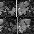 Approach to Detection and Characterization of Hepatic Hemangiomas
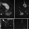
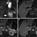 Resonance Imaging of Adenocarcinoma of the Pancreas
 Imaging of the Liver
 Self-Parameterized Active Contours for Medical Image Segmentation with Emphasis on Abdomen
 Imaging with VHF Signal Generation: A New Contrast Mechanism for Cancer Imaging Over Large Fields of View
 Liver Segmentation Without Prior Statistical Models


(14)
(15)
. A R (k 1,k 2,k 3) and A F (k 1,k 2,k 3) are amplitude components, and and are phase components. The normalized cross spectrum is defined as(16)
between r(n 1,n 2,n 3) and f(n 1,n 2,n 3) is the 3D inverse DFT (3D IDFT) of
Related posts:
Approach to Detection and Characterization of Hepatic Hemangiomas
Resonance Imaging of Adenocarcinoma of the Pancreas
Imaging of the Liver
Self-Parameterized Active Contours for Medical Image Segmentation with Emphasis on Abdomen
Liver Segmentation Without Prior Statistical Models
Stay updated, free articles. Join our Telegram channel
Full access? Get Clinical Tree
