Prostate Cancer Localization with Multiparametric Magnetic Resonance Imaging

ADC

k _ep

k _el

IAUC30

IAUC60

IAUC90

0.6438

0.5210

0.2044

Preprocessing and Ground Truth

Multispectral MRI dataset used in this chapter consists of three different types of MR images per the preliminary feature selection study. Each multispectral component represents a particular anatomical and functional response of the prostate gland. Feature vectors used for segmentation are intensity values of multispectral MR images. For each type of multispectral MR images, a single slice of size 256 × 256 from a 3D MRI is chosen by clinicians to be used in our experiments. The prostate consists of various zones such as transition zone (TZ) and peripheral zone (PZ). However, only the PZ region is considered since 70 % of the prostate cancer occurs in this region [26]. Several other studies presented their sensitivity/specificity results using only PZ region as well [3, 8]. A manual registration was implemented for each patient to align the PZ region across different image types. All images are median filtered using a 3 × 3 window to improve signal-to-noise ratio, remove the spikes, and suppress possible registration errors. For each of the multispectral images, applying a simple transformation to the intensity values normalized PZ region intensities. Normalization is applied such that intensities in the PZ region had zero mean and unit standard deviation for all the training and testing subjects for a particular multispectral image. Then,

${Y}_{{}_{ij}}=\frac{X_{{}_{ij}}-{\mu}_j}{\sigma_i}$

(1)

where X _ijis the image type i for patient j, Y _ijis the normalized image type i for patient j, and μ _j, σ _irefers to the mean and standard deviation of multispectral image type i. This brings intensities of different types of MR images within the same dynamic range, improving the stability of the classifiers. The ground truth is obtained based on pathology. A radiologist transfers the tumor regions on the histological slides to the MR images by viewing the histological slides, ex vivo MR images of these slides, and in vivo MR images. True-positives and true-negatives are defined on a pixel basis, providing a considerable amount of data points for evaluation.

Segmentation Methods

Multispectral MR images show a discernible intensity difference that differentiates between cancerous and normal tissue. Therefore, intensity values of anatomical and functional images are used as our features to construct the classifiers. In the following sections, we present a comparison of the performance of several classification methods, SVM, C-SVM, and the proposed cost-sensitive CRF. A total of 21 patients are used in the training and testing steps. During the experiments, based on the ground truth obtained from pathology, leave-one-out cross validation is implemented using twenty subjects for training and one subject for testing for each of the 21 subjects.

The support vector machine (SVM) is a universal supervised learning algorithm based on statistical learning theory [17]. Learning is the process of selecting the best mapping function f(x,w) from a set of mapping models parameterized by a set of parameters w ∈ Ω, given a finite training dataset (x _i,y _i) for i = 1, 2, …, N, where x _i∈ R ^dis a d-dimensional input (feature) vector, y _i∈ {−1, 1} is a class label, and N is the number samples in the training dataset. The objective is to estimate a mapping function f(x → y) in order to optimally classify future test samples. Suppose we have a mapping that separates the set of positive samples from negatives. This amounts to finding weights w and the bias b such that

$$$ {y}_i<w,{x}_i>+b>0\kern1em \mathrm{for}\kern1em i=1,2,\dots, N $$ ” src=”/wp-content/uploads/2016/03/A303895_1_En_22_Chapter_Equ2.gif”></DIV></DIV><br /> <DIV class=EquationNumber>(2)</DIV></DIV></DIV><br /> <DIV class=Para>If there exists a hyperplane satisfying (<SPAN class=InternalRef><A href=$ 2), the set is said to be linearly separable. For a linearly separable set, it is always possible to rescale w and b in (2) such that

$$$ {y}_i<w,{x}_i>+b\ge 1\kern1em \mathrm{for}\kern1em i=1,2,\dots, N $$ ” src=”/wp-content/uploads/2016/03/A303895_1_En_22_Chapter_Equ3.gif”></DIV></DIV><br /> <DIV class=EquationNumber>(3)</DIV></DIV></DIV><br /> <DIV class=Para>In this way, closest training point to the dataset has a distance of <SPAN id=IEq10 class=InlineEquation><IMG alt=$ . Among the alternative hyperplane that satisfy (3), SVM selects the one for which the distance to the closest point in the training data is maximal. Since the distance to the closest point is $1/\left\Vert w\right\Vert$ , SVM finds the hyperplane by minimizing ${\left\Vert w\right\Vert}^2$ under constraints given by (3). The quantity $2/\left\Vert w\right\Vert$ is called the margin; hence, SVM is called a maximum margin classifier. When the classes are not linearly separable, constraints are relaxed by adding nonnegative slack variables (ξ ₁, ξ ₂, …, ξ _N) in the formulation of the optimization problem. The optimum classifier can be found by solving

$$$ \kern0.5em \begin{array}{ll} \min \hfill & \hfill \frac{1}{2}{\left\Vert w\right\Vert}^2+C{\displaystyle \sum_{i=1}^N{\xi}_i}\hfill \\ {}\hfill \mathrm{st}.\hfill & \hfill {y}_i\left(<w,{x}_i>+b\right)\ge 1-{\xi}_i\kern1em \mathrm{for}\kern1em i=1,2,\dots, N\hfill \\ {}\hfill \hfill & \hfill {\xi}_i\ge 0\kern1em \mathrm{for}\kern1em i=1,2,\dots, N\hfill \end{array} $$ ” src=”/wp-content/uploads/2016/03/A303895_1_En_22_Chapter_Equ4.gif”></DIV></DIV><br /> <DIV class=EquationNumber>(4)</DIV></DIV></DIV><br /> <DIV class=Para>where <SPAN class=EmphasisTypeItalic>C</SPAN> is the weight for the penalty term for misclassifications. SVM is a frequently used algorithm in image classification applications [<CITE><A href=$ 19, 27] with several variations. In this study, we use the υ-SVM since selection of υ is easier than alternatives [28]. The υ-SVM has the following primal formulation:

$$$ \begin{array}{ll} \min \hfill & \hfill \frac{1}{2}{\left\Vert w\right\Vert}^2-\upsilon +{\displaystyle \sum_{i=1}^N{\xi}_i}\hfill \\ {}\hfill \mathrm{st}.\hfill & \hfill {y}_i\left(<w,{x}_i>+b\right)\ge 1-{\xi}_i\kern1em \mathrm{for}\kern1em i=1,2,\dots, N\hfill \\ {}\hfill \hfill & \hfill {\xi}_i\ge 0\kern1em \mathrm{for}\kern1em i=1,2,\dots, N\hfill \end{array} $$ ” src=”/wp-content/uploads/2016/03/A303895_1_En_22_Chapter_Equ5.gif”></DIV></DIV><br /> <DIV class=EquationNumber>(5)</DIV></DIV></DIV><br /> <DIV class=Para>In prostate cancer localization, however, there is a disadvantage to <SPAN class=EmphasisTypeItalic>υ</SPAN>-SVM formulation since it penalizes errors of both classes equally [<CITE><A href=$ 28]. A reformulation of (5) is called 2υ-SVM, given by

$$$ \begin{array}{ll} \min \hfill & \frac{1}{2}{\left\Vert w\right\Vert}^2-\upsilon +\frac{\gamma}{N}{\displaystyle \sum_{i\in {I}_{+}}{\xi}_i}+\frac{1-\gamma}{N}{\displaystyle \sum_{i\in {I}_{-}}{\xi}_i}\hfill \\ {}\hfill \mathrm{st}.\hfill & \hfill {\mathrm{y}}_i\left(<w,{x}_i>+b\right)\ge 1-{\xi}_i\kern1em \mathrm{for}\kern1em i=1,2,\dots, N\hfill \\ {}\hfill \hfill & \hfill {\xi}_i\ge 0\kern1em \mathrm{for}\kern1em i=1,2,\dots, N\hfill \end{array} $$ ” src=”/wp-content/uploads/2016/03/A303895_1_En_22_Chapter_Equ6.gif”></DIV></DIV><br /> <DIV class=EquationNumber>(6)</DIV></DIV>where <SPAN class=EmphasisTypeItalic>γ</SPAN> ∈ [0,1] is a parameter controlling the trade-off between false-negatives and false-positives and <SPAN class=EmphasisTypeItalic>I</SPAN> <SUB>+</SUB>, <SPAN class=EmphasisTypeItalic>I</SPAN> <SUB>−</SUB> are the numbers of training samples that belong to the positive and negative classes, respectively. Solution to above primal formulation is obtained by transforming this convex optimization problem into a corresponding dual formulation resulting in a quadratic cost function. 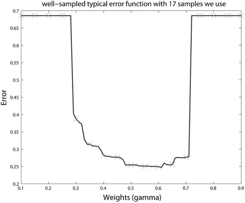Two parameters in linear 2<SPAN class=EmphasisTypeItalic>υ</SPAN>-SVM that determine the classifier performance, <SPAN class=EmphasisTypeItalic>γ</SPAN> and <SPAN class=EmphasisTypeItalic>υ</SPAN>, are selected as explained next.</DIV><br /> <DIV class=Para>Optimal parameter selection in SVM [<CITE><A href=$ 29, 30] is crucial to classifier effectiveness. However, optimal SVM parameters certainly differ depending on the defined error criterion. 2υ-SVM parameter selections require a full grid search over υ and γ values to reach the optimum parameters. SVM trained in this way will be referred throughout as C-SVM. One study [13] proposed a variant of coordinate descent algorithm that would speed up the search process. However, due to non-smoothness of the probability of positive and probability of false-negative values, the proposed accelerated algorithm could not be applied in this study. The parameter υ was searched in the range [0.01, 0.50] over 50 points, and γ was searched in the range [0.10, 0.90] over 17 points, respectively. These resolutions are chosen in an ad hoc manner based on experience related to the smoothness of the underlying function. Increasing the number of sampling points of υ and γ may result in slightly better estimates; however, it would be a computationally intensive task not producing significant differences given typical error functions. Figure 1 shows such a typical error vs. weights values of a single value with 17 samples we use. Notice that minima would not change significantly when the number of samples is increased.

Fig. 1

Error rate vs. γ (weights) of a single υ value with 17 sampling points we use

In this study, we utilize and compare three different training methodologies. In our experiments, we implemented 2υ-SVM with the linear kernel based on our preliminary investigation. We trained the 2υ-SVM using cross validation to determine the optimal υ and γ parameters. Now, we describe the proposed training schemes that are used to choose υ and γ parameters.

The objective of the first training method is to minimize the number of pixel misclassifications from both classes. A full grid search is conducted on υ and γ parameters to find the lowest error rate. SVM trained by this method will be referred to as SVM₁ for classical SVM and C-SVM₁ for C-SVM. In the second training method, optimal υ and γ parameters are obtained by performing a full grid search, where υ and γ are selected such that detection probability is maximized while constraining false-positive probability to be below a threshold value referred to as SVM₂ for classical SVM and C-SVM₂ for C-SVM. Third training method utilizes area under the ROC curve (AUC) metric to assess the performance of a classifier. For each υ and γ pair in the grid, Platt’s function is used to convert SVM decisions into posterior probabilities [26, 27], and ROC curves are obtained using these posterior probabilities. SVM trained by this method are similarly referred as SVM₃ for classical SVM and C-SVM₃ for C-SVM.

Bias Selection. In the training stage, we determine the optimal υ and γ pair to be used in testing process using one of the training methods mentioned above. However, to make a fair comparison between classical and C-SVM classifiers, the bias of each constructed classifier is adjusted to achieve a false-positive rate of 0.30 for the training dataset. This bias adjustment is performed for all classical SVM and cost-sensitive C-SVM classifiers during the training and not changed for individual test subjects. The false-positive rate used is selected based on a clinically acceptable performance.

Even though SVM benefits from the maximum margin property, it does not utilize spatial information in the classification process. Therefore, we propose a new segmentation method that uses CRF in a cost-sensitive framework as described next. CRF was proposed initially by Lafferty et al. [31] in the context of segmentation and labeling of 1D text sequences. Similar to MRF, it is used to model the spatial interaction in images. For an observed data x and corresponding labels y, MRF models the posterior probability using Bayes’ rule:

$p\left(y\Big|x\right)\propto p\left(x,y\right)=p\left(x\Big|y\right)p(y)$

where the prior over the labels is assumed to be stationary and Markovian and likelihood is assumed to have a factorized form $p\left(x\Big|y\right)={\displaystyle \prod_{i\in S}p\left({x}_i\Big|{y}_i\right)}$ where S is the set of nodes. Recently, it has been noted [22] that a factorized form of the likelihood model is too restrictive in certain image classification applications because label interactions do not depend on the observed data. Therefore, CRF directly models the posterior probability distribution p(y|x) for a given input image sample x and label y using a Gibbs prior model. Before we present the CRF definition as stated in [31], we first restate the notation. Suppose that the observed features from a given training image are given by x = {x _i}_{i ∈ S}where x _i∈ R ^dis the feature vector for node i. Corresponding labels at image nodes are given by y = {y _i}_{i ∈ S}. CRF constructs a discriminative conditional model p(y|x) from the jointly distributed observations x and y, and the prior, p(y), is not modeled explicitly.

CRF Definition. Let G = (S, E) be a graph such that the vertices of G index y. Then (y, x) is said to be a conditional random field if, when conditioned on x, the random variables y _iobey the Markov property with respect to the graph: $p\left({y}_i,x\Big|{y}_{S-\left\{i\right\}}\right)=p\left({y}_i,x\Big|{y}_{S-{N}_i}\right)$ where S-{i} is the set of all nodes in the graph except the node i, N _iis the set of neighbors of the node i in G, and y _Ωrepresents the set of labels at the nodes in the set Ω [31].

Recently, another study [22] introduced a two-dimensional extension of CRF by using the local discriminative models to capture the class associations at individual nodes as well as the interactions on the neighboring nodes for a 2D graph:

$p\left(y\Big|x\right)=\frac{1}{Z} \exp \left\{{\displaystyle \sum_{i\in S}A\left({y}_i,x\right)+{\displaystyle \sum_{i\in S}{\displaystyle \sum_{j\in {N}_i}V\left({y}_i,{y}_j,x\right)}}}\right\}$

(7)

where Z is a normalizing constant known as the partition function, A(y _i,x) is the node potential at node i, and V(y _i,y _j,x) is the edge potential between nodes i and j that encourages spatial smoothness. The terms A(y _i,x) and V(y _i,y _j,x) can be seen as unary data term and smoothness term, respectively. Node potential A(y _i,x) is a measure of how likely the node i will take label y _igiven image node x ignoring the effects of other node labels in the image. Generalized linear models are used extensively in statistics to model the class posterior given the observations. In our formulation, A(y _i,x) is modeled using a local discriminative model that outputs the association of the node i with class y _i:

$A\left({y}_i,x\right)= \ln \left(\frac{1}{1+ \exp \left(-{y}_i{w}^Tx\right)}\right)$

(8)

where w is the normal to the linear decision boundary that is obtained from C-SVM as explained next in more detail. The edge potential is a function of all observations of x. The aim of the smoothness term is to have similar labels at a pair of nodes for which the node value supports such a hypothesis. For a pair of neighboring nodes (i, j), let μ _ijdenote a new feature vector obtained by taking the absolute difference of x _iand x _j, μ _ij= [1, |x _i− x _j|], where x _iis simply chosen to be the pixel intensity at node i.

$V\left({y}_i,{y}_j,x\right)={y}_i{y}_j{\kappa}^T{\mu}_{ij}$

(9)

and κ contains the model parameters. The first component of μ _ijis fixed to one to accommodate the bias parameter. In summary, the node potential acts as a unary term for individual nodes, while the edge potential is a data-dependent discriminative label interaction (smoothness term). In the classical approach to constructing (7), the parameters of the node potential w and edge potential κ are determined jointly in the training stage, where they are initialized with logistic regression and randomly, respectively [21]. However, in a recent study, we have shown that this approach does not result in accurate prostate cancer segmentation [16].

Therefore, in this chapter, node potential parameter w is obtained from SVM, and edge potential parameter κ is estimated subsequently. Use of a standard maximum-likelihood approach to learn κ parameter involves the evaluation of partition function Z. In general, evaluation of Z is considered as an NP-hard problem [21]. Therefore, we resort to approximation method, pseudo likelihood, to estimate the κ parameter. In this study, we adopted pseudo likelihood [32] to estimate κ due to its simplicity and efficiency. In the pseudo likelihood approach, the factored approximation is

$\overset{\wedge }{\kappa }=\underset{\kappa }{ \arg\;\max}\;{\displaystyle \sum_m{\displaystyle \sum_i \ln\;p\left({y}_i^m\Big|{y}_{N_i}^m,{x}^m,\kappa \right)}}$

(10)

where κ refers to the neighbors of the node i and y _i^mis the observed label for node i in the m th training image. Further, (10) can be expressed as shown in (11), where τ is regularization constant. To ensure that the log likelihood is convex and prevent over-fitting due to the pseudo likelihood approximation, we assign a Gaussian prior on κ with zero mean and covariance τ ² I, where I is the identity matrix. Then we compute the local consistency parameters using its penalized log likelihood:

$\overset{\wedge }{\kappa }=\underset{\kappa }{ \arg\;\max}\;{\displaystyle \sum_{m=1}^M{\displaystyle \sum_{i\in S}\left\{ \ln \left(\delta \left({y}_i{w}^Tx\right)\right)+{\displaystyle \sum_{j\in {N}_i}{y}_i{y}_j{\kappa}^T{\mu}_{ij}(x)- \ln \left({Z}_i^m\right)}\right\}-\frac{1}{2{\tau}^2}{\kappa}^T\kappa }}$

(11)

where

${Z}_i={\displaystyle \sum_{y_i\in \left\{-1,1\right\}}\left\{ ln\left(\delta \left({y}_i{w}^Tx\right)\right)+{\displaystyle \sum_{j\in {N}_i}{y}_i{y}_j{\kappa}^T{\mu}_{ij}(x)}\right\}}$

When τ, chosen by cross validation, is given, the penalized likelihood in (11) is quadratic with respect to κ. Therefore, (11) is convex and can be maximized using a simple gradient descent algorithm. Note that node potentials act as a constant in this optimization process.

Finally, for a given test image x, we perform mean-field inference [33] using the estimated model parameters w and κ to obtain an optimal label configuration y. Next, we describe the multispectral MRI dataset used in this study and present the results obtained using the methods that were described.