Fig. 1
Block diagram of the proposed system for tumor characterization and classification; the blocks outside the dotted shaded rectangular box represent the flow of off-line training system, and the blocks within the dotted box represent the online real-time system
In this section, we describe, in detail, the image acquisition procedure and the various techniques used for feature extraction and selection and classification.
Patients and Image Acquisition
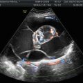
Twenty women (age: 29–74 years; mean ± SD = 49.5 ± 13.48) were recruited for this study. The study was approved by the Institutional Review Board. The procedure was explained to each subject and informed consent was obtained. Among these 20 women, 11 were premenopausal and 9 were postmenopausal. All these patients were consecutively selected during presurgical evaluation by one of the authors of this paper (blinded for peer review). Patients with no anatomopathological evaluation were excluded from the study. Biopsies indicated that among the 20 patients, 10 had malignancy in their ovaries and 10 had benign conditions. Postoperative histology results indicated that the benign neoplasms were as follows: 5 endometriomas, 2 mucinous cystadenoma, 1 cystic teratoma, 1 pyosalpinx, and 1 serous cyst. The malignant neoplasms were as follows: 3 primary ovarian cancers (undifferentiated carcinomas), 3 borderline malignant tumors, 1 krukenberg cancer, 1 serous cystadenocarcinoma, 1 serous carcinoma, and 1 carcinosarcoma. All patients were evaluated by 3D transvaginal ultrasonography using a Voluson-I (GE Medical Systems) according to a predefined scanning protocol using 6.5 MHz probe frequency (Thermal Index: 0.6 and Mechanical Index: 0.8). A 3D volume of the whole ovary was obtained. The acquired 3D volumes were stored on a hard disk (Sonoview™, GE Medical Systems). Volume acquisition time ranged from 2 to 6 s depending on the size of the volume box. In cases where a given adnexal mass contained more than one solid area and, hence, had more than one volume stored, only the volume best visualizing the mass was chosen for further analysis. Figure 2 shows typical ultrasound images of benign and malignant classes. We chose the middle 100 images from each volume from each subject. Thus, the evaluated database consisted of 1,000 benign images and 1,000 malignant images.
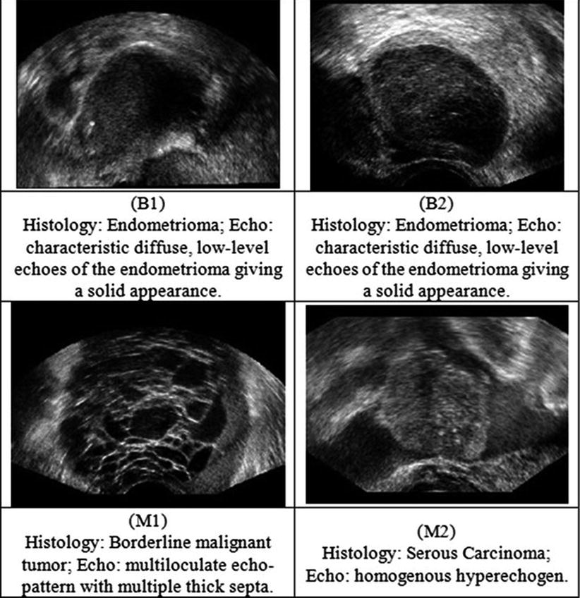
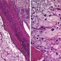
Fig. 2
Ultrasound images of the ovary: (B1–B2) benign conditions, (M1–M2) malignant tumor
Feature Extraction
Feature extraction is one of the most important steps in an automated CAD system. It was observed that the type of tumor (tumor-like lesions, benign, tumors of low malignant potential, and malignant) was correlated with lesion diameter, with larger tumors more likely to be malignant [26]. Moreover, there are several morphological changes in the benign and malignant ultrasound images [27, 28]. Usually the histopathologic cytoarchitecture of malignant tumors is different from benign neoplasm with several areas having intra-tumoral necrosis [29]. These changes in lesion diameter and cytoarchitecture variations manifest as nonlinear changes in the texture of the acquired ultrasound images. Therefore, in this work, we have extracted features based on the textural changes in the image and also nonlinear features based on the higher-order spectra information. In this section, we describe these features in detail.
Texture Features
Texture features measure the smoothness, coarseness, and regularity of pixels in an image. The extracted texture descriptors quantify the mutual relationship among intensity values of neighboring pixels repeated over an area larger than the size of the relationship [30, 31]. There are several texture descriptors available in the literature [31]. We have chosen the following features:
Deviation
Let f(i) where (i = 1, 2, …, n) be the number of points whose intensity is i in the image and A x be the area of the image. The occurrence probability of intensity i in the image is given by  The standard deviation is given by
where μ = mean of intensities.
The standard deviation is given by(1)
Fractal Dimension (FD)
Theoretically, shapes of fractal objects remain invariant under successive magnification or shrinking of objects. Since texture is usually a scale-dependent measure [32], using fractal descriptors can alleviate this dependency. A basic parameter of a fractal set is called the fractal dimension (FD). FD indicates the roughness or irregularity in the pixel intensities of the image. Visual inspection of the benign and malignant images in Fig. 2 shows that there are differences in the regularity of pixel intensities in both classes. We have hence used FD as a measure to quantify this irregularity. The larger the FD value, the rougher the appearance of the image. Consider a surface S in Euclidean n-space. This surface is self-similar if it is the union of N r nonoverlapping copies of itself scaled up or down by a factor of r. Mathematically, FD is computed [33, 34] using the following formula:
(2)
In this work, we used the modified differential box counting with sequential algorithm to calculate FD [34]. The input of the algorithm is the grayscale image where the grid size is in the power of 2 for efficient computation. Maximum and minimum intensities for each (2 × 2) box are obtained to sum their difference, which gives the M and r by

where M = min(R, C), s is the scale factor, and R and C are the number of rows and columns, respectively. When the grid size gets doubled, R and C reduce to half of their original value and above procedure is repeated iteratively until max(R, C) is greater than 2. Linear regression model is used to fit the line from plot log(N r ) vs. log(1/r) and the slope gives the FD as
(3)
(4)
Gray-Level Co-occurrence Matrix (GLCM)
The elements of a Gray-Level Co-occurrence Matrix (GLCM) are made up of the relative number of times the gray-level pair (a, b) occurs when pixels are separated by the distance (a, b) = (1, 0). The GLCM of an m × n image can be defined by [35]
where (a,b), (a + Δx, b + Δy) ∈ M × N, d = (Δx, Δy). | ⋅ | denotes the cardinality of a set. The probability of a pixel with a gray-level value i having a pixel with a gray-level value j at a (Δx, Δy) distance away in an image is
(5)
(6)
We calculated the following features:
![$$ Entropy(E)=-{\displaystyle \sum}_i{\displaystyle \sum}_j{P}_d\left(i,j\right)\times ln\left[{P}_d\left(i,j\right)\right] $$](/wp-content/uploads/2016/09/A301939_1_En_26_Chapter_Equ7.gif)
(7)
(8)
Higher-Order Spectra (HOS)
Second-order statistics can adequately describe minimum-phase systems only. Therefore, in many practical cases, higher-order correlations of a signal have to be studied to extract information on the phase and nonlinearities present in the signal [38–41]. Higher-order statistics denote higher-order moments (order greater than two) and nonlinear combinations of higher-order moments, called the higher-order cumulants. In the case of a Gaussian process, all cumulant moments of order greater than two are zero. Therefore, such cumulants can be used to evaluate how much a process deviates from Gaussian behavior. Prior to the extraction of HOS-based features, the preprocessed images are first subjected to Radon transform [42]. This transform determines the line integrals along many parallel paths in the image from different angles θ by rotating the image around its center. Hence, the intensities of the pixels along these lines are projected into points in the resultant transformed signal. Thus, the Radon transform converts a 2D image into a 1D signal at various angles in order to enable calculation of HOS features. This 1D signal is then used to determine the bispectrum, B(f 1 , f 2 ), which is a complex valued product of three Fourier coefficients given by
![$$ B\left({f}_1,{f}_2\right)=E\left[A\left({f}_1\right)A\left({f}_2\right){A}^{*}\left({f}_1+{f}_2\right)\right] $$](/wp-content/uploads/2016/09/A301939_1_En_26_Chapter_Equ10.gif)
where A(f) is the Fourier transform of a segment (or windowed portion) of a single realization of the random signal a(nT), n is an integer index, T is the sampling interval, and E[·] stands for the expectation operation. A *(f 1 + f 2 ) is the conjugate at frequency (f 1 + f 2 ). The function exhibits symmetry and is computed in the nonredundant/principal domain region Ω as shown in Fig. 3. We calculated the H parameters that are related to the moments of bispectrum. The sum of logarithmic amplitudes of bispectrum H 1 is
(10)
(11)
Fig. 3
Principal domain region (Ω) used for the computation of the bispectrum for real signals
The weighted center of bispectrum (WCOB) is given by
where i and j are frequency bin index in the nonredundant region.
(12)
We extracted H 1 and two weighted center of bispectrum features for every one degree of Radon transform between 0° and 180°. Thus, the total number of extracted features would be 724 (181 × 3). To summarize, the following are the steps to calculate the HOS features from the ultrasound image [36]: (1) The original image is first converted to 1D signal at every 1° angle using Radon transform. (2) The 256 point FFT is performed with 128 point overlapping to maintain the continuity. (3) The bispectrum of each Fourier spectrum is computed using the Eq. (9). Similarly, the bispectrum is determined for every 256 samples. (4) The average of all these bispectra gives one bispectrum for every ultrasound image. (5) From this average bispectrum, the moments of bispectrum and weighted center of bispectrum features given in Eqs. (11) and (12) are calculated.
Feature Selection
After the feature extraction process, there were a total of 729 features (5 texture based and 724 HOS based). Most of these features would be redundant in information they retain, and using them to build classifiers would result in the curse of dimensionality problem [22] and over fitting of classifiers. Therefore, feature selection is done to ensure that only unique and informative features are retained. In this work, we have used Student’s t–test [43] to select significant features. Here, a t-statistic, which is the ratio of difference between the means of the feature for two classes to the standard error between class means, is first calculated, and then the corresponding p-value is calculated. A p-value that is less than 0.01 or 0.05 indicates that the means of the feature are statistically significantly different for the two classes, and hence, the feature is very discriminating. On applying the t-test, we found that many features had a p
Table 1
Classifier performance measures
SVM kernel | TP | TN | FP | FN | Accuracy (%) | Sensitivity (%) | Specificity (%) | PPV (%) |
|---|---|---|---|---|---|---|---|---|
Linear | 100 | 99 | 0 | 1 | 99.8 | 99.61 | 100 | 100 |
Polynomial (order 1) | 100 | 100 | 0 | 0 | 99.8 | 99.6 | 100 | 100 |
Polynomial (order 2) | 100 | 100 | 0 | 0 | 99.5 | 100 | 99.9 | 99.9 |
Polynomial (order 3) | 100 | 100 | 0 | 0
Related posts: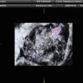 Benign Sex Cord-Stromal Tumors: Clinical and Ultrasound Features Benign Sex Cord-Stromal Tumors: Clinical and Ultrasound Features
 Ovarian Tumors: Computed Tomography and Magnetic Resonance Ovarian Tumors: Computed Tomography and Magnetic Resonance
 and MR Imaging of Malignant Germinal and Stromal Ovarian Tumours and MR Imaging of Malignant Germinal and Stromal Ovarian Tumours
 and MR of Benign Ovarian Germ Cell Tumours and MR of Benign Ovarian Germ Cell Tumours
 Ovarian Tumors (Serous/Mucinous/Endometrioid/Clear Cell Carcinoma): Clinical Setting and Ultrasound Appearance Ovarian Tumors (Serous/Mucinous/Endometrioid/Clear Cell Carcinoma): Clinical Setting and Ultrasound Appearance
 Histopathology Histopathology
Stay updated, free articles. Join our Telegram channel
Full access? Get Clinical Tree
 Get Clinical Tree app for offline access

|