Fig. 1.1
First ever human head image using MRI at 0.1 T from EMI Central Research Laboratories. For this image CT-type “back projection” was used. (Courtesy of Ian Young and first published in an article from the November, 1978 issue of New Scientist magazine)
MRI Principles
The science behind MRI is far from intuitive and the detailed physics are outside the purview of this chapter. However, a solid foundation is important for understanding the various MRI neuroimaging methods . To that end, the core concepts and terminology are reviewed here.
The Proton
At its core, MRI involves the interaction of several sources of electromagnetism , which include those inherent to the machine as well as those intrinsic to the organism being studied. Extending NMR principles we could gather information from the nuclei of a multitude of molecules within a given sample, provided that they have an odd number of protons, have a spin, and are mobile enough to change direction. However, in clinical MRI, there is a focus on the hydrogen nuclei. This is primarily due to its abundance in the body, mostly in the form of water, but also in various other forms such as fat. Each hydrogen atom’s nucleus is comprised of a single proton. The positively charged proton is naturally spinning on its axis which, by the rules of electromagnetism, results in the creation of tiny magnetic fields. In essence, each proton acts as a tiny bar magnet with a specific strength and directionality (i.e., they are vectors). However, with their random orientations and movements there is usually no net magnetic effect. It is the composite magnetic activity of numerous protons with which we are interested and the smallest volume of tissue (or voxel) that is measured to eventually produce the final MR image, comprising the net effect of trillions of protons within a single cubic millimeter (1 mm3).
The Static External Magnetic Field (B0)
The most powerful source of electromagnetism arising from the MRI is the static magnetic field to which the subject is exposed in the center of the machine, which in short-hand is called B0 (“B-nought”). As with the proton magnetic fields, B0 is a vector and the strength of this field is inherent for a given machine as measured in Tesla (T), with most clinical machines currently at the 1.5 T strength. The so-called “high-field” MRI is also becoming widespread at levels of 3 T and greater, which has some important implications that will be addressed later. Although B0 is a static field in the sense that it persists throughout the entirety of the acquisition process, it is important to note that it is not completely uniform and there are tiny variations in the magnetic field (i.e., it has inhomogeneities). This latter property has multiple implications, as it affects the quality of the final images and it also underlies the concepts of T2 and T2* (“T2-star”).
As the subject is exposed to B0, their protons are influenced in two main ways. First, the previously randomly oriented tiny magnetic vectors of the protons become aligned in the same plane as B0 and obtain a net directionality along that axis. This novel orientation of the protons net vector is known as longitudinal magnetization . The second outcome is that the protons gain a type of motion known as “precession ,” in which each proton moves gyroscopically (i.e., similar to a wobbling top). The precession (or “resonant”) frequency for the protons is characteristic for a given B0, increasing with higher field strengths. We can temporarily alter B0 by several means and it is the resultant variable frequency of the protons, which fundamentally makes MRI possible. The above conditions of longitudinal magnetization and precession can be considered an equilibrium state from which other parts of the MRI acquisition process can be understood.
The Radiofrequency (RF) Pulse
A second source of electromagnetism , known as the radiofrequency (RF) pulse , is then administered from an RF coil at a specific frequency (i.e., resonant frequency). There are usually multiple RF pulses administered during an acquisition process which can vary in their angles with respect to B0 (e.g., 90°, 180°, etc.) and the predetermined interval of their occurrence, the variable effects of which will become clearer when we touch upon specific sequence protocols. The initial pulse is usually known as an “excitation pulse” and we can first consider the outcome of this. Upon receiving the appropriate frequency of RF pulse, the given groups of protons absorb energy and are excited into two important reactions that occur simultaneously. First of all, the protons’ magnetic field vector rotates away from the equilibrium plane of B0, such that there is no longer a net longitudinal magnetization. Secondly, the movements of the protons are harmonized, such that their precession frequencies are now in-sync (“in-phase”) with each other or have “phase-coherence” and the protons now have a net transverse magnetization. In the presence of B0, it is actually the dynamic state of this net transverse magnetization that produces a radiowave and induces a current in a RF coil (usually different from the one that transmitted the RF pulse) that eventually leads to an MR signal from the tissues of interest.
T1, T2, and T2*
Soon after administration of the RF excitation pulse , the protons begin giving off absorbed energy to their local molecular environment (known as their “lattice”) and their vectors eventually return to the plane of B0, reestablishing longitudinal magnetization. When plotted over time, you can see that this relaxation process occurs exponentially and the measured time constant of this up-sloping curve is called T1, which is characteristic for given tissues and will therefore vary between voxels. This process is known equivalently as longitudinal, T1 or spin-lattice relaxation .
Occurring simultaneously is a process involving loss of phase-coherence of the precessing protons that, in distinction from above, involves an exchange of energy between protons (instead of the environment). As mentioned, B0 has slight field strength inhomogeneities and the local magnetic environment experienced by each group of protons is also inherently inhomogeneous. Together these processes contribute to reestablishing the protons variable precession frequencies, i.e., they undergo “dephasing” and a net reduction of transverse magnetization a process known as free induction decay (FID) . The process of energy exchange between protons is known equivalently as “spin-spin” or T2 relaxation . This component can be isolated by temporarily eliminating B0 inhomogeneities, which is one of the other functions of RF pulses in spin-echo (SE)-based techniques. The resultant relaxation effects are plotted over time and the time constant of the exponentially decaying curve is called T2, which again is characteristic for given tissues and will vary between voxels.
The composite process of FID, encompassing the contributions of both spin-spin and B0 inhomogeneities is described by the time constant T2*. T2* relaxation can result in rapid dephasing of the transverse magnetization which decreases the strength of the echo signal and can lead to clinically useless images. It is for this reason that it is often desirable to suppress T2* effects. However, at other times it is desirable to accentuate T2* effects, leading to greater conspicuity of certain tissues among other uses to be detailed later.
By convention, tissues with shorter T1 relaxation time constants appear as higher signal intensity (e.g., fat and white matter), while those with longer ones have lower signal intensity. Conversely, longer T2 relaxation time constants appear as higher signal intensity (e.g., cerebrospinal fluid (CSF)) while shorter ones have lower signal intensity. Further details of what determines the particular T1 and T2 of the different tissues (both normal and pathologic) can be found in any comprehensive MRI text, with characteristic tissue signals summarized in Table 1.1. The most important point to remember is that the variability of the time constants between different tissues determines their signal intensities and the differences in signal intensities between the voxels in a sample of interest; therefore, represent the contrast in our final images. In general terms, it is established that T1 effects give better anatomic information, while T2 effects can be more useful for evaluation of pathology—with much overlap in practice.
Table 1.1
Differentiation of tissue type based upon MRI weighting and signal intensities
Weighting | Signal intensity | Tissue examples |
|---|---|---|
T1 | Dark | Air |
Fast-flowing blood | ||
Mineral rich tissue (e.g., cortical bone) | ||
Low | High free-water content (e.g., edema, CSF) | |
Intermediate | Proteinaceous tissue | |
Bright | Fat | |
Blood products (intracellular metHb) | ||
Slow-flowing blood | ||
T2 | Dark | Air |
Fast-flowing blood | ||
Mineral-rich tissue (e.g., cortical bone) | ||
Low | Bone islands | |
Intermediate | Fat | |
Bright | High free-water content (e.g., edema, CSF) | |
Proteinaceous tissue | ||
Blood products (oxyHb, extracellular metHb) |
Virtually in all MRI images, the independent effects of T1 and T2 are each contributing to various degrees, but the greatest contrast in our images is obtained by maximizing the difference between the time constants of the various tissues. It is the responsibility of neuroimagers to maximize the clinical utility of the images, which includes independently promoting T1 or T2 weighting and dividing these into different imaging series to interpret their effects separately. In order to increase the contributions by either T1 or T2 effects, we “weight” the images by selecting parameters that will give us the greatest differences in signal intensity between tissues of interest (i.e., contrast). For a given sequence, we can choose how long after the excitation pulse we want the MR to initialize the “readout” of the echo signals, a parameter known as echo time (TE) as well as the time between subsequent excitation pulses, a parameter known as repetition time (TR) . Essentially, a short TR setting (400–800 ms) in conjunction with a short TE setting (5–30 ms) will yield tissue contrast that emphasizes differences in T1 signal, while a long TR will minimize the differences in T1 signal. An appropriately long TE setting (60–120 ms) will emphasize tissue differences in T2 signal; however, the TE must not be too long, because the progressively weakening T2 signal will eventually result in poor image quality. As you will see, we can also affect the resultant images by adjusting other parameters in the various sequence protocols.
Gradients, K-Space, and the Fourier Transformation
Gradients are an additional source of electromagnetism administered from other coils in the MRI and can be utilized in a variety of ways via the same basic effect: temporarily altering B0 in a predictable manner. One important use of gradients is in their pulsatile application along the different axes of B0 contributing to slice selection, frequency encoding, and phase encoding of the protons. An abstract concept called k-space is essentially a 2D matrix representing the raw frequency-encoded and phase-encoded data derived from the steps above. In some basic sequence protocols, k-space is filled row-by-row, requiring multiple repetitions of the acquisition steps to populate the entire matrix. The end result of a complicated interaction between the RF pulses and gradients will be a spatially encoded MR signal in this form.
Even though each voxel is uniquely encoded by the steps above, it is actually a single-summed signal (i.e., the “bulk magnetization”), which is detected in MRI. In order to convert this raw data into useful images, it is necessary to disentangle the signal; this is done by breaking it down into its component frequencies, an automated process that is dictated by the mathematical algorithm known as the Fourier Transformation . With the culmination of the above steps, we have established our final images that have been imparted with spatial information and signal intensities that contrast the tissues of interest in our subject.
Conventional MRI Sequence Protocols
Since the early days of conventional MRI , a multitude of pulse sequence protocols (or “protocols” as they will be referred to) have been developed. Although the same basic principles are utilized, each of the protocols differs in the details of acquisition as well as in the final product and therefore their specific utility in neuroimaging . Some protocols allow for faster acquisition times, improved image quality, or even accentuation of various tissue contrasts. There is usually a compromise with the various MRI protocols and creating a balance of the best possible signal, contrast, and spatial resolution in the shortest possible time is a basic goal of the neuroimager. Fortunately, many of these can be acquired and interpreted in combination for a given patient, contributing to MRIs flexibility in clinical applications. Although there are hundreds of different protocols with a variety of acronyms, we will focus on some of the core protocols in generic categories.
Spin-Echo (SE)
Spin-Echo (SE) was the most commonly used protocol during the infancy of MRI and it continues to have specific utility. The defining acquisition characteristic for SE protocols come from the application of an initial 90° RF excitation pulse followed by a 180° RF “refocusing pulse ,” with a couple of relevant consequences. First of all, this creates a focused SE signal measured at time TE, which leads to the population of a single line of the k-space matrix during each TR cycle (i.e., between excitation pulses). Also, as previously alluded to, the RF refocusing pulse neutralizes contributions from T2* effects, which allows for a “true T2” signal.
Adjustments of the TR and TE are the parameters utilized in SE to T1 or T2 weight the resultant images. Because each TR in basic SE sequences results in population of only a single line of k-space , the TR cycle must be repeated numerous times and is the most time-consuming parameter. Therefore, TR is set to as short as possible which, along with a short TE, results in T1 weighting. Thus, the greatest clinical utility of basic SE protocols reside in the creation of T1-weighted images, while acquisition of T2-weighted images can be time prohibitive and other protocols have been developed to allow for this (Fig. 1.2).
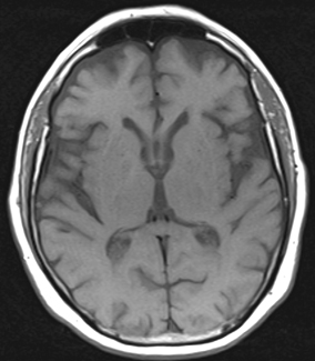
Fig. 1.2
T1 SE axial image obtained at 1.5 T, TR of 570 and TE of 17
Fast Spin-Echo (FSE)
The utility of Fast Spin-Echo (FSE) protocols comes mainly from their improved acquisition efficiency. This is accomplished by various alterations to the basic SE protocol with respect to the RF pulses and spatial encoding steps. These alterations usually include a rapidly repeating refocusing pulse, which yields a series of SE signals (or an “echo train”) that are subjected to different encoding gradients, allowing for population of multiple lines of k-space during each single TR. Therefore, in FSE there are additional parameters under our control, including the number of SEs to be produced during a given TR known as the “echo train length” (ETL) , which directly contributes to the rapidity of acquisition. The SE signals in FSE are also each recorded at different TEs; so, this adjustable parameter is actually known as “effective TE.”
Building upon their slower predecessor, FSE protocols have become ubiquitous in modern neuroimaging . In addition to the reduced acquisition time, FSE protocols can also improve image quality. Signal contributions from T2* effects are further minimized by the repetitive refocusing pulses. However, these faster protocols also have their own disadvantages including potentially higher signal from certain tissues (e.g., fat and CSF), which can limit evaluation of parenchyma particularly at the skull base and periventricular regions. These limitations can be largely addressed by complementary methods as we will see shortly in Fig. 1.3.
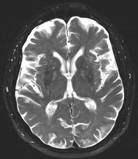
Fig. 1.3
T2 FSE axial image obtained at 1.5 T, TR of 5,370 and TE of 111
Gradient Recalled Echo (GRE)
Another group of protocols known generically as gradient recalled echo (GRE) offer even faster acquisition times than the various SE techniques, but this is at the cost of potentially noisier images. This sequence differs from SE techniques by the potential use of partial flip angles (i.e., less than 90°) as well as the use of gradients (applied bidirectionally) to dephase and then rephase transverse magnetization and form a gradient-echo signal. So, the adjustable parameters in GRE include TR and TE as well as the choice of the particular partial flip angle. Partial flip angles result in less substantial tipping of the protons’ magnetic vectors from the longitudinal plane and therefore faster recovery of full longitudinal magnetization allowing for shorter TRs. Without the use of the refocusing RF pulse, it is also possible to measure the echo signal sooner than in SE protocols (i.e., the TE can be shorter). However, this also yields preservation of T2* effects, which can result in signal loss and geometric distortion. These T2* (or “magnetic susceptibility”) effects can especially limit evaluation in areas with different tissue types abutting one another, for example, at the interface of air and soft tissues at the paranasal sinuses. Conversely, GRE can exploit these T2* effects, for example, allowing easier detection of certain tissues such as blood. Therefore, the utility of GRE protocols in conventional MRI lies in the rapid acquisition of T1-weighted images and these “T2-like” images. As we will see, T2* effects are also important for some of the advanced MRI techniques (Fig. 1.4).
< div class='tao-gold-member'>
Only gold members can continue reading. Log In or Register to continue
Related posts:

Stay updated, free articles. Join our Telegram channel

Full access? Get Clinical Tree


